Calc1131W9T3 - de Casteljau Bezier curves

Tuesday, 1 May 2018

8:30 PM

Machine generated alternative text:
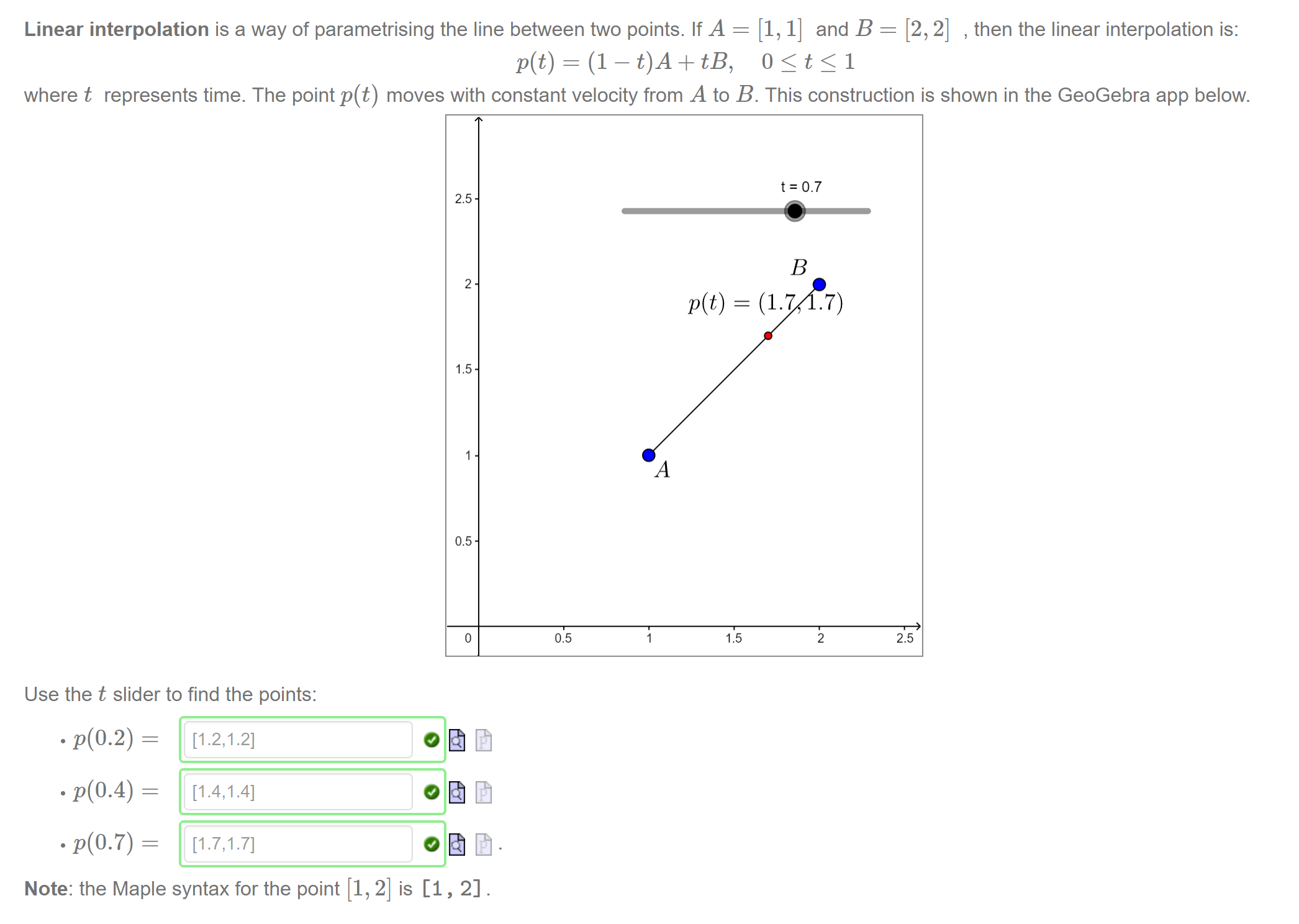
Linear interpolation is a way of parametrising the line between two points. If A = [1, 1] and B = [2, 2] , then the linear interpolation is: 
p(t) 
= (1 — + tB, 0 s t S 1 
where t represents time. The point p(t) moves with constant velocity from A to B. This construction is shown in the GeoGebra app below. 
2.5 
1.5 
0.5 
0.5 
t=O.7 
= (1.7 .7) 
1.5 
2.5 
Use the t slider to find the points: 
• p(o.2) 
• p(0.4) 
• p(o.7) 
[1.2, 1.2] 
[1.7,1.7] 
Note: the Maple syntax for the point [1,


Machine generated alternative text:
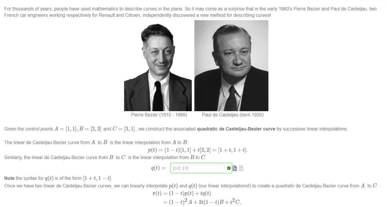
For thousands of years; people have used mathematics to describe curves in the plane. So it may come as a surprise that in the early 1960's Pierre Bezier and Paul de Casteljau, two 
French car engineers working respectively for Renault and Citroen, independently discovered a new method for describing curves' 
Pierre Bezier (1910 - 1999) 
Paul de Casteijau (born 1930) 
Given the control points A = [1, 1], B = [2, 2] and C = [3, 1] , we construct the associated quadratic de Casteljau-Bezier curve by successive linear interpolations. 
The linear de Casteljau-Bezier curve from A to B is the linear interpolation from A to B: 
Similarly, the linear de Casteljau-Bezier curve from B to C is the linear interpolation from B to C 
Note the syntax for q(t) is of the form [1 + t, 1 — t]. 
Once we have two linear de Casteljau-Bezier curves; we can linearly interpolate p(t) and q(t) (our linear interpolations') to create a quadratic de Casteljau-Bezier curve from A to C 
r(t) 
= (1 — + tq(t) 
= (1 - t)2A + 2t(1 - + Pc.


Machine generated alternative text:
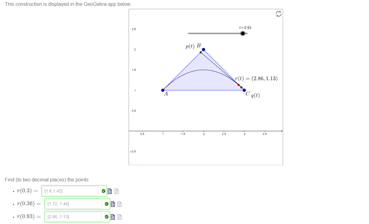
This construction is displayed in the GeoGebra app below: 
p(t) B 
Find (to two decimal places) the points 
t=093 
r(t) = (2.86, 1.13) 
• r(0.3) 
• r(0.36) — 
• r(0.93) — 
[1 72, 1.46] 
[286, 1<3]


Machine generated alternative text:
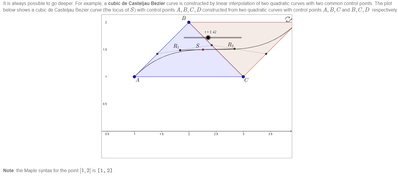
It is always possible to go deeper For example, a cubic de Casteljau Bezier curve is constructed by linear interpolation of two quadratic curves with two common control points The plot 
below shows a cubic de Casteljau Bezier curve (the locus of S) with control points A, B, C, D constructed from two quadratic curves with control points A, B, C and B, C, D respectively. 
t=042 
s 
Note: the Maple syntax for the point [1, 2] is [1, 2]


Machine generated alternative text:
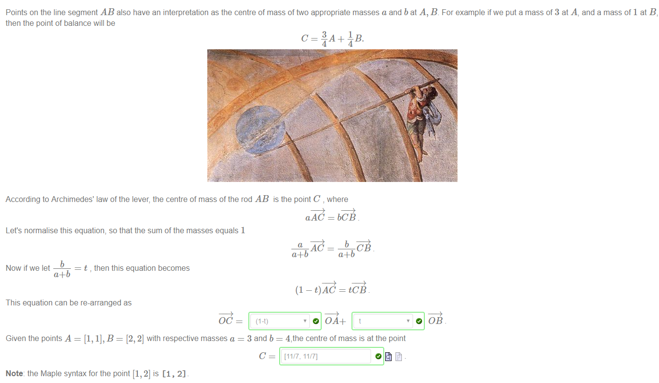
Points on the line segment AB also have an interpretation as the centre of mass of two appropriate masses a and b at A, B. For example if we put a mass of 3 at A, and a mass of 1 at B i 
then the pont of balance will be 
According to Archimedes' law of the lever, the centre of mass of the rod AB is the point C , where 
Let's normalise this equation, so that the sum of the masses equals 1 
Now if we let 
t then this equation becomes 
This equation can be re-arranged as 
OC 
Given the points A = [1, 1], B = [2, 2] with respective masses a 
Note: the Maple syntax for the point [1, 2] is [1, 2] 
aAC = bCB 
CB 
(1 - t)AC = tCB 
4, the centre of mass is at the point 
[11/7: 11/7] 
0 0B 
3 and b 
C


Machine generated alternative text:
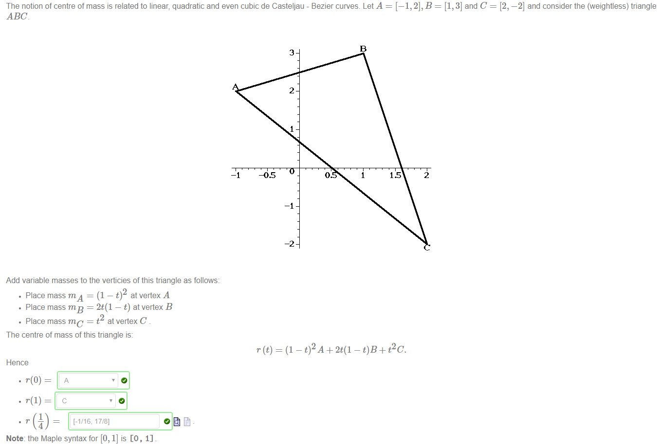
The notion of centre of mass is related to linear; quadratic and even cubic de Casteljau - Bezier curves. Let A 
= [1,3] and C 
= [2, —2] and consider the (weightless) triangle 
ABC 
Add variable masses to the verticies of this triangle as follows: 
• Place mass m A = (1 —t) at vertex A 
• Place mass = 2t(1 — t) at vertex B 
• Place mass mc = t at vertex C 
The centre of mass of this triangle is: 
Hence 
Note: the Maple syntax for [0, 1] is [O, 1] 
3 
2 
-2 
= (1 — + 2t(1 - 0B + pc. 
2


Machine generated alternative text:
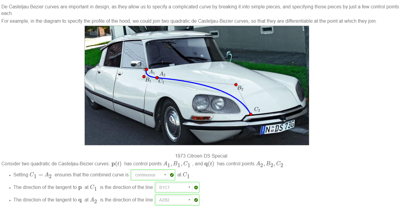
De Casteljau Bezier curves are important in design, as they allow us to specify a complicated curve by breaking it into simple pieces, and specifying those pieces by just a few control points 
each 
For example, in the diagram to specify the profile of the hood, we could join two quadratic de Casteljau-Bezier curves7 so that they are differentiable at the point at which they join 
4. 
1973 Citroen DS Special 
Consider two quadratic de Casteljau-Bezier curves: p(t) has control points Al , Bl, Cl and q(t) has control points .42, B2, C2 
• Setting Cl = 242 ensures that the combined curve is continuous 
• The direction ofthe tangent top at Cl is the direction ofthe line 
• The direction ofthe tangent toq at 142 is the direction ofthe line 
O at Cl 
SICI 
A2B2


Machine generated alternative text:
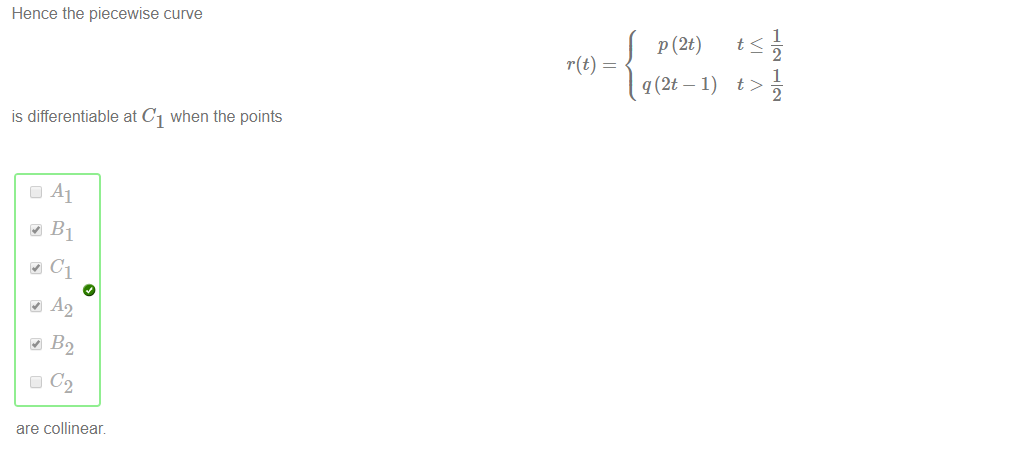
Hence the piecewise curve 
p (2t) 
r(t) 
q(2t- 1) 
is differentiable at Cl when the points 
Al 
are collinear 
1 
1


Created with Microsoft OneNote 2016.