Calc1131W7T3 - Piecewise differentiable curves
Saturday, 21 April 2018
11:24 AM
Created with Microsoft OneNote 2016.
![Untitled picture.png Machine generated alternative text:
Let g(x)
—1
—4x +5m — 1 and h@)
From these two functions we can construct a new piecewise defined function, such as
g(x) if x S 2
f@)
h(x) if x > 2.
Even though g and h are continuous and differentiable, we must check if the combined function is continuous and differentiable at the point in which they meet, in this case x
To check continuity means to check that the left-hand limit, the right-hand limit and the function value are all equal Namely that
lim f (x) = lim = f(2).
In the example,
lim_ f@)
lim f (ET) =
So the function f
O continuous at x = 2.
Similarly we check that f is differentiable at x = 2. Formally this means that the limit lim
exists. We can take a shortcut since g and h are differentiable at x
The limit lim
h
does not
O exist.
Note: we need check continuity as well as differentiability to determine that a piecewise function as above is differentiable at a point.
Untitled picture.png Machine generated alternative text:
An artist draws a straight line through the points A
point C = [4, 0].
You advise a function of the form
The function should satisfy the conditions:
and the differential condition
05
= 0] and B
[1, 1]. The artist would like to choose a pleasant function to smoothly continue this line in the fashion of a trajectory to the
2
f@)
2
3
ax2 + + c.
These conditions uniquely determine the coefficients as
-2.5/9
19/18](Calc1131W7T3%20-%20Piecewise%20differentiable%20curves_files/image001.png)
![Untitled picture.png Machine generated alternative text:
An artist draws a straight line through the points A
point C = [4, 0].
You advise a function of the form
The function should satisfy the conditions:
and the differential condition
05
= 0] and B
[1, 1]. The artist would like to choose a pleasant function to smoothly continue this line in the fashion of a trajectory to the
2
f@)
2
3
ax2 + + c.
These conditions uniquely determine the coefficients as
-2.5/9
19/18
Untitled picture.png Machine generated alternative text:
Consider the functions
.T2 — 5/2C + 5/2
defined on the interval (0, 1], and the functions
cost x)
• k(x) —2m —1
• t(x)
defined on the interval (1, 2).
Select all pairs of functions which can be piecewise combined into a differentiable function in the interval (O, 2)
Cl fand j
Cl fand k
fand t
Cl g and j
Cl g and k
Cl g and t
h and j
h and k
h and C
𝑓𝑥=𝑎𝑥2+𝑏𝑥+𝑐
𝑓1=𝑎×12+𝑏×1+𝑐=1
> 𝑎+𝑏+𝑐=1
𝑓4=𝑎×42+𝑏×4+𝑐=0
>16𝑎+4𝑏+𝑐=0
> 𝑓′1=2𝑎𝑥+𝑏=0.5
// Equate the three equations to get 𝑎, 𝑏 and 𝑐.](Calc1131W7T3%20-%20Piecewise%20differentiable%20curves_files/image002.png)
![Untitled picture.png Machine generated alternative text:
Consider the functions
.T2 — 5/2C + 5/2
defined on the interval (0, 1], and the functions
cost x)
• k(x) —2m —1
• t(x)
defined on the interval (1, 2).
Select all pairs of functions which can be piecewise combined into a differentiable function in the interval (O, 2)
Cl fand j
Cl fand k
fand t
Cl g and j
Cl g and k
Cl g and t
h and j
h and k
h and C
Untitled picture.png Machine generated alternative text:
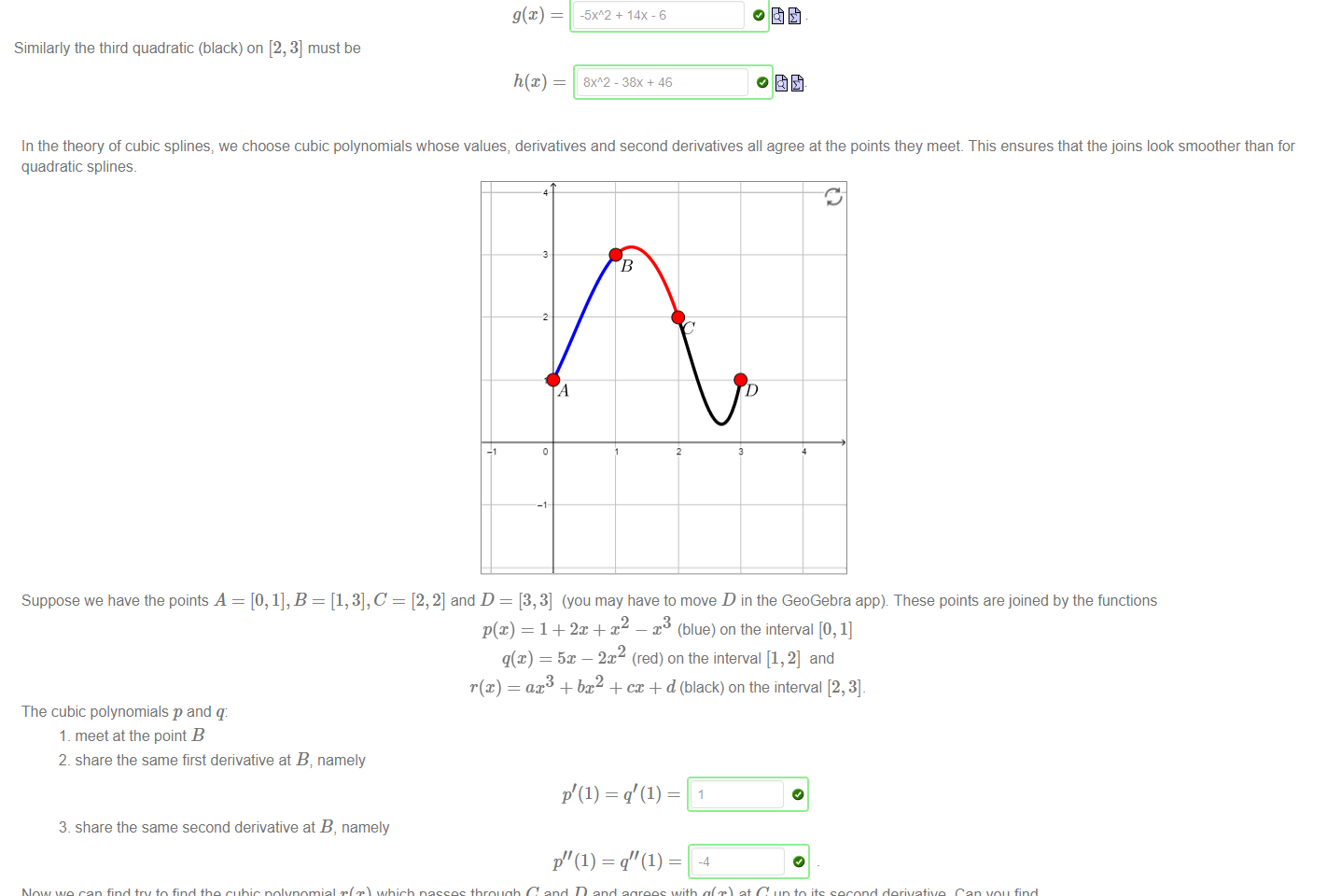
In the theory of splines, we try to find simple (quadratic or cubic) curves that pass through given points, and fit together to form smooth (differentiable) curves. Suppose we want to fit quadratic
curves together through the points A = [0, 1], B = [1, 3], C = [2, 2] and D = [3, 4]_
Move the points C and D in the GeoGebra app below to their specified locations
Let's suppose the first quadratic (blue) is given by f@) = 2m + 1 on the interval [0, 1]. You can easily verify that the curve passes through points A and B.
Our second quadratic (red) is of the form
ax2 + c
and must pass through points B and C and have the same derivative as f@) at B (remember to move C to the point [2, 2]). Then
+ 14X-6
Similarly the third quadratic (black) on [2, 3] must be](Calc1131W7T3%20-%20Piecewise%20differentiable%20curves_files/image003.png)