Calc1131W7T1 - Counting real zeros with the IVT

Saturday, 21 April 2018

11:24 AM

Machine generated alternative text:
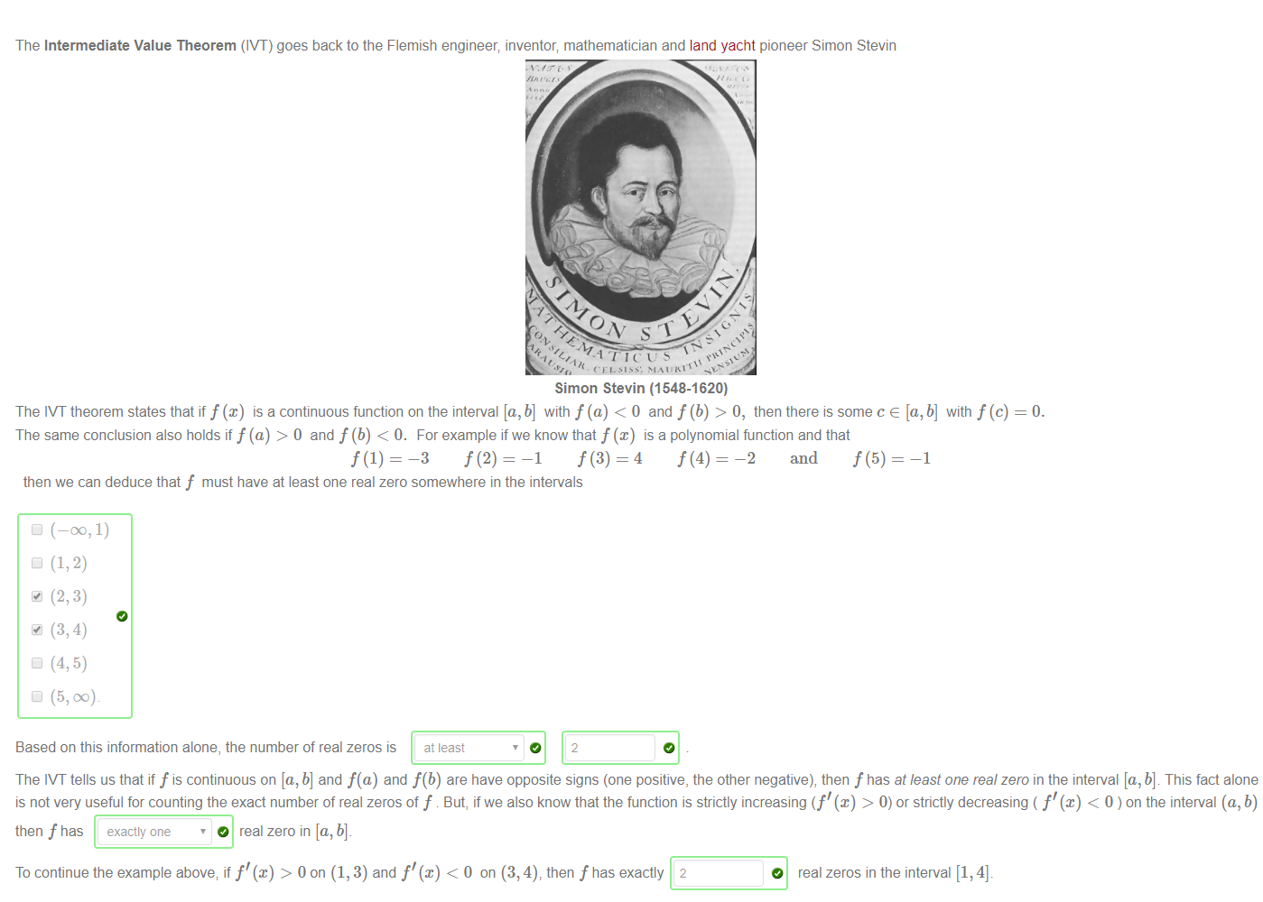
The Intermediate Value Theorem (IVT) goes back to the Flemish engineer; inventor; mathematician and land yacht pioneer Simon Stevin 
Simon Stevin (1548-1620) 
The 'VT theorem states that iff@) is a continuous function on the interval [a,b] with f (a) < 0 and f (b) > O, then there is some c e [a,b] with f(c) 
The same conclusion also holds if f(a) > 0 and f (b) < 0. For example if we know that f (x) is a polynomial function and that 
f(2) — 
f(4) — 
—2 and f (5) 
—3 
—1 
—1 
then we can deduce that f must have at least one real zero somewhere in the intervals 
(—00, 1) 
(5, DC) 
Based on this information alone, the number of real zeros is at least 
The 'VT tells us that if f is continuous on [a, b] and f(a) and f(b) are have opposite signs (one positive, the other negative), then f has at least one real zero in the interval [a, b] This fact alone 
is not very useful for counting the exact number of real zeros of f . But, if we also know that the function is strictly increasing (f' (x) > 0) or strictly decreasing ( f'@) < 0 ) on the interval (a, b) 
then f has 
To continue the example above, if f'@) > 0 on (1, 3) and f'@) < 0 on (3, 4), then f has exactly 2 
O real zeros in the interval [1, 4].


Machine generated alternative text:
A differentiable function f@) is said to be increasing on the interval I when it is either strictly increasing f' (x) > 0 or constant f'@) = O for all x e I. A increasing function preserves order in 
the sense that bigger function input results in bigger function output: 
if a, b e I and a b then f(a) f(b)_ 
Similarly a function f(x) is said to be decreasing on the interval I when it is either strictly decreasing f' (x) < 0 or constant f'@) = O for all x e L A decreasing function preserves the order in 
the sense that bigger function input results in smaller function output: 
if a, b e I and a bthen f(a) 2 f(b) 
A increasing or decreasing function on I is called monotonic on I. In the special case when I = Domain(f) t we usually replace "on I " with "evemvhere't For example f(x) 
x IS Increasing 
a = 28 
b = 88 
f2(u 
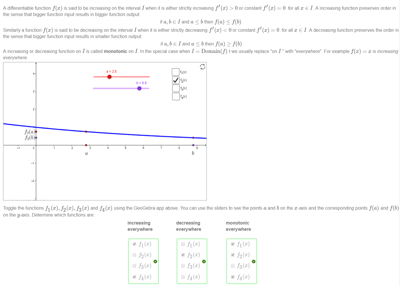
Toggle the functions fl@), h f3 (x) and f4 (x) using the GeoGebra app above. You can use the sliders to see the points a and b on the x-axis and the corresponding points f(a) and f(b) 
on the y-axis. Determine which functions are: 
Increasing 
everywhere 
f2(x) 
Cl f3(x) 
f4(x) 
decreasing 
everywhere 
f2(x) 
Cl f3(x) 
f4(x) 
monotonic 
everywhere 
f2(x) 
Cl f3(x) 
f4(x)


Machine generated alternative text:
Consider the polynomial p@) 
The derivative of p is 
8x + 7 shown below 
-20 
300 
200 
100 
-100 
-200 
-300 
10 
20 
By factoring this derivative and looking at the points [—10, p(—10)] and [10, p(10)], we see there are three regions where p is monotonic 
increasing 
• decreasing 
increasing 
Notice that 
O on the interval [— 
O on the interval [ 
• P(-IO) — -439/3 < o 
. p(2) = 
. p(10) 
= 1081/3 > o 
By applying the IVT to p on three intervals, we conclude that p(x) has exactly 3 
O real roots. 
Note we need to introduce two extra points [—10, [10, p(10)] because the IVT can not be applied directly to an infinite interval (—00,


Machine generated alternative text:
How many zeros does f(x) 
A sensible guess might be 2 
cos(aræ) have in the interval I 
= [14, 16] 
14 
15 
16 
O How do you know there are not more? We can use the IVT and monotonic functions to find out 
We would like to use the IVT on intervals where f@) is monotonic. The function f is not monotonic on I, but we can break I into two subintervals Il U 12 — I where f is monotonic on Il and 
separately monotonic on 12 
Since f'@) 
• decreasing on the interval Il — 
• increasing on the interval 12 
O , the function is 
[14, 15] 
[15,161 
We apply the IVT for f on these intervals separately Since f@) is continuous on the interval Il and 
• f(14) — 
• f(15) — 
then by the IVT there is at at least one zero in this interval. Since the function is monotonic on Il there is exactly one zero in the interval Il 
Similarly, f(x) is continuous on the interval 12 and 
• f(15) — 
• f(16) — 
Then by the 'VT there is at least one zero in 12_ Since the function is monotonic on 12 there is exactly one zero in 12 _ Hence the number of zeros in the interval I 
expected _ 
Note the Maple syntax for the interval [l,ff] is [1, pi) 
Il LJ 12 is exactly as we


Machine generated alternative text:
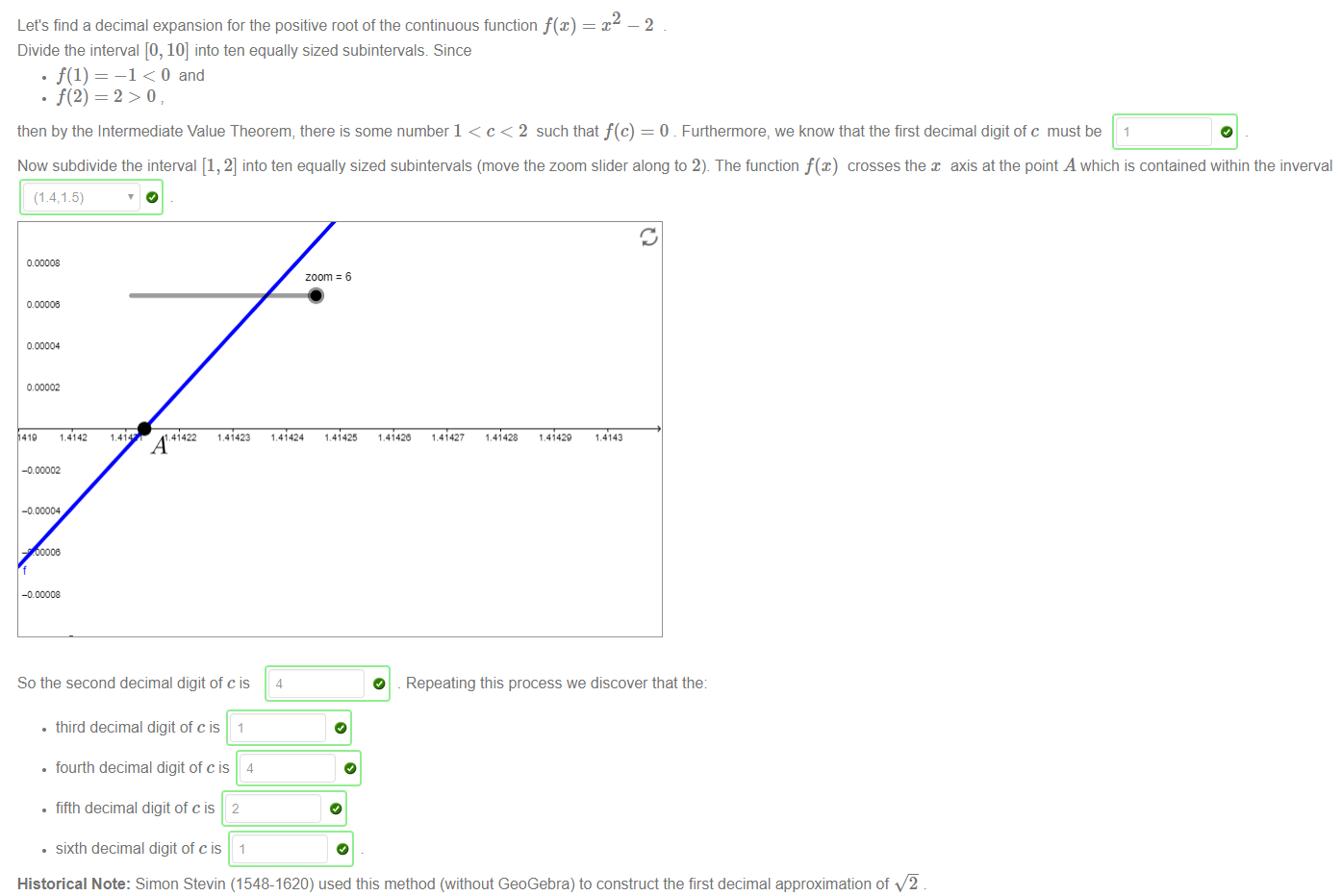
Let's find a decimal expansion for the positive root of the continuous function f@) 
Divide the interval [0, 10] into ten equally sized subintervals. Since 
—1 < 0 and 
2 
—2 
then by the Intermediate Value Theorem, there is some number 1 < c < 2 such that f(c) = 0 . Furthermore, we know that the first decimal digit of c must be 
Now subdivide the interval [1, 2] into ten equally sized subintervals (move the zoom slider along to 2). The function f(x) crosses the x axis at the point A which is contained within the inverval 
(1.4:1 5) 
1.4142 
,41422 
1.41423 
zoom 6 
1.41425 
1.41424 
4 
1.41428 
1.41429 
So the second decimal digit of c is 
• third decimal digit of cis 1 
• fourth decimal digit of cis 4 
• fifth decimal digit of cis 2 
• sixth decimal digit of cis 1 
O 
Repeating this process we discover that the 
Historical Note: Simon Stevin (1548-1620) used this method (without GeoGebra) to construct the first decimal approximation of v'ä


Created with Microsoft OneNote 2016.