Project - Report
Contents
This report continues the experimentation and formulation of a wireless signal strength to distance algorithm as conceived here
Assessment of Preliminary Findings
In the preliminary report, the graphs of logarithmic averages were generated with error.
Microsoft Excel's x-axis was set to display values logarithmically - however this did not properly scale the graph to show a linear best fit, as suggested from the Linear Regression analysis results.
This was resolved by reverting the display mode of the x-axis to a linear scale, and plotting $log_{10}(x)$ instead of $x$ along the x-axis.
| Indoor | Outdoor | |
|---|---|---|
| Previous | 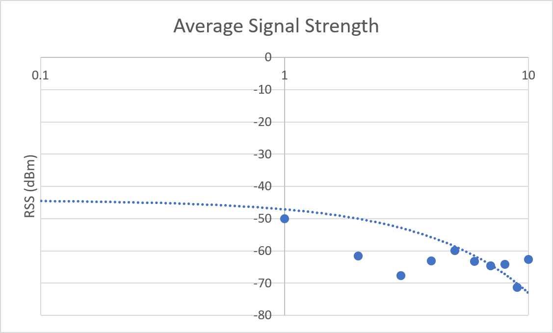 | 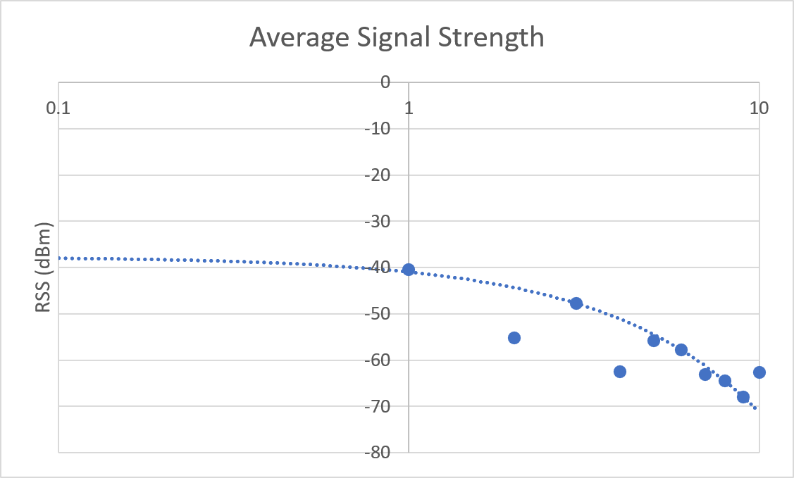 |
| Corrected | 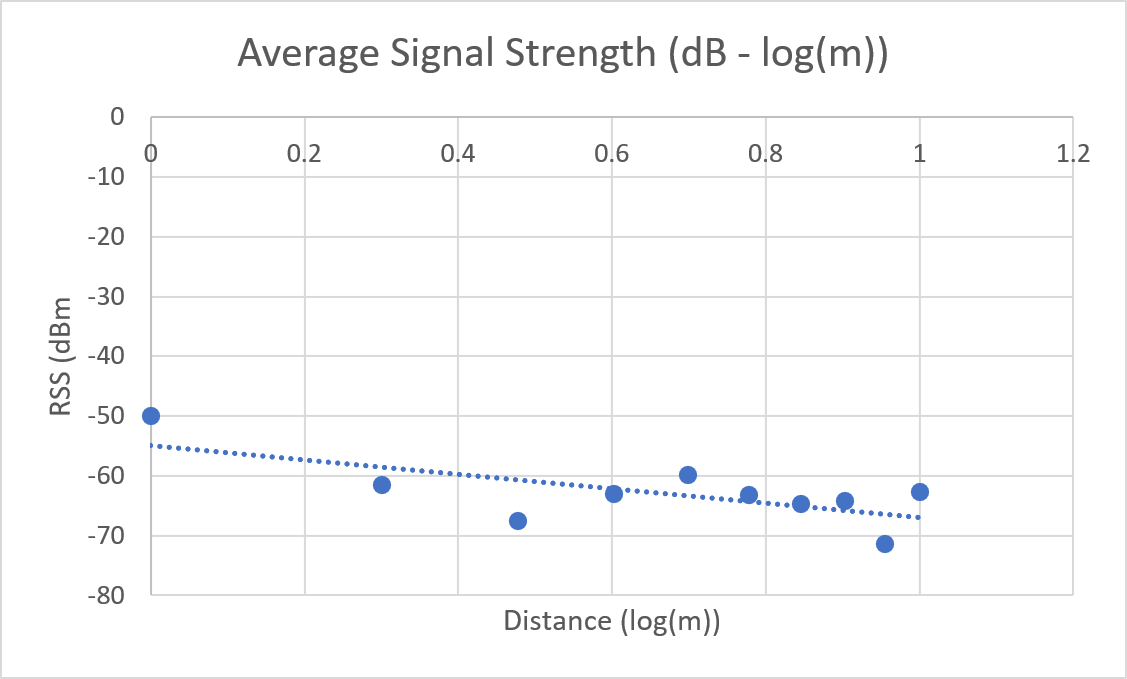 | 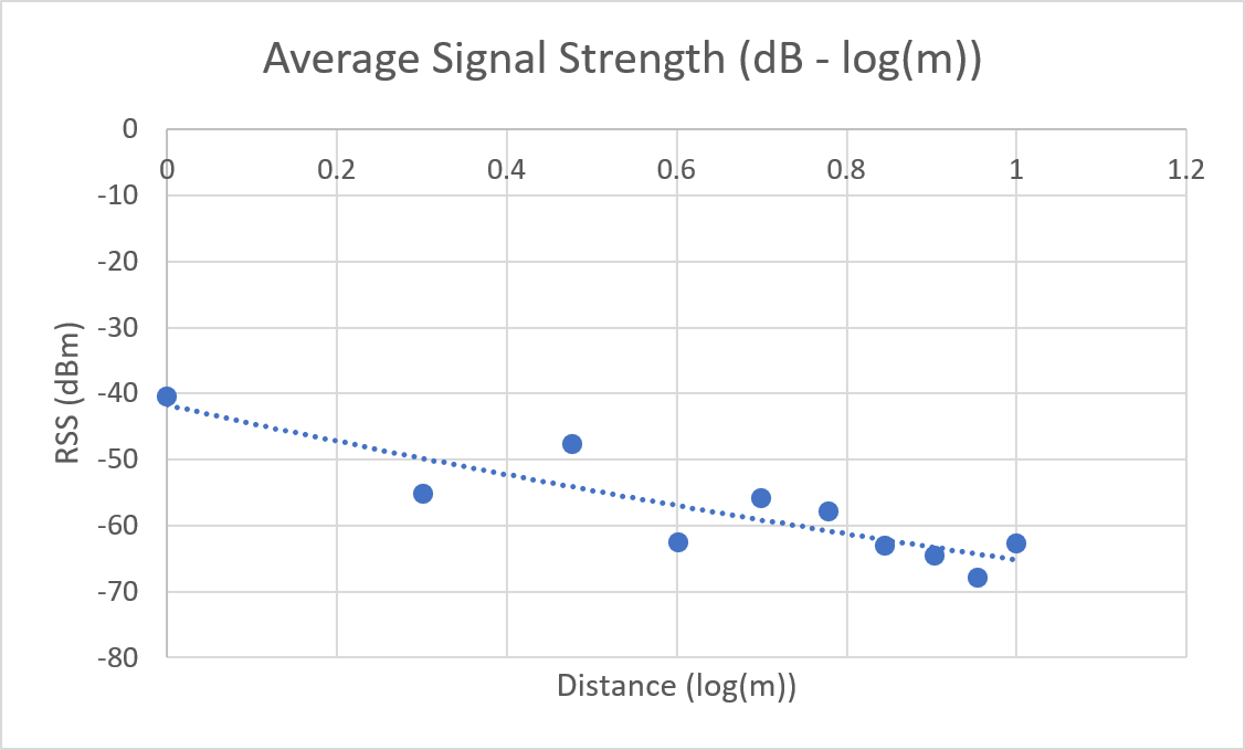 |
In extension of the other conclusions drawn from the preliminary report, the data set for indoor environment measurements will be discarded, as they were deemed too noisy to use.
Effects of multipath transmission (i.e. radio waves reflecting off walls) and interference from other indoor devices attribute to the weak $R^2$ value of $0.38$, compared to the outdoor environment's $R^2$ value of $0.62$.
Distance Estimation using Wireless Signal Strength
Abstract
A Log-Distance Model is derived from samples of wireless signal strengths recorded in an outdoor environment. Sample data is cleaned with a Kalman Filter and outlier data group removal, which improved the accuracy of the model.
In comparison to the naive distance estimation presented in the preliminary report, the new model demonstrates a higher hit-accuracy against all distance classes from the test sample. Whilst RSSI values are not a great metric for distance estimation, they can be used within reasonable accuracy.
Introduction
The evolution of technology has paved way for the ever increasing need of wireless communication.
From the early origins of mobile phone calls, to GPS, to Remotely Operated Machinery, to IoT - wireless technologies have been crucial in the modern age.
Geospatial coordination systems have become crucial for many wireless applications, where it is often useful to locate an object in an area. These include, but are not limited to: asset tracking, navigation systems, and heat mapping.
However, implementation of a such system can be challenging, due to the large variety of environmental factors and infrastructural costs that may be required. This report aims to find a universal and portable method of determining distances between two devices.
Related Works
Geopositioning
Time of Arrival
It is possible to determine the distance between two radio devices by exploiting the properties of electromagnetic waves - in particular the relationship between a wave's frequency and velocity.
$$ v = f\lambda $$
By determining the time delta between the transmission and reception of a wireless signal, the distance can be calculated.
This is however, impractical due to the need of a high accuracy clock circuit that is costly in terms of price but also energy usage. Implementing such an algorithm is unviable as it will decrease the runtime of battery powered devices.
Sea of Sensors
Anchor-based solutions exist - where statically positioned devices (separated at fixed distances) are used to locate a device.
A grid of access points/stations can be deployed in an area, such that a given radio device coincides with several of the station's pickup radius. By calculating the RSS values at each station, trilateration can be performed to determine the position of a device in the area. This can be likened to a GPS system, where a GPS device receives beacons from satellites orbiting the Earth to locate itself.
Whilst this solution is viable in an office/corporate environment, it is costly to implement due to the density of stations needed. Due to the reliance of stations to determine distance, this solution will not work in public/district/rural areas.
Distance Modelling
Free Space Propagation Model
$$ strength = \frac{k}{d^2} $$ $$ FSL = 20 log(d) + 20 log(f) + 32.45 $$
At f = 2.4 GHz, $FSL = PL_0 + 10 n log(d)$
The free space model defines the simplest scenario for the propagation of a radio signal.
The energy of a signal decays proportionally to the inverse square of their separation.
This model relies on the assumption that both the transmitter and receiver have line of sight (LOS) positioning, with no obstacles between them.
2 Ray Model
$$ TGNL = PL_0 + 10 n log(d) - 32 $$
At distances past $d_{br} = 10\ m$, the two-ray path model can be used, which accounts for reflections of radio waves
Multiwall Model
$$ MWL = PL_0 + 10 n log(d) + \sum_{i} L_{W_i} $$
The multiwall model factors in specific losses for each medium that a ray travels through.
Log-Distance / Log Normal Shadowing Model
$$ PL = PL_0 + 10 n log(d/d0) + \chi $$
This model extends the free space model, opening scope to paths that are obstructed between the transmitter and receiver.
Egli's Model
$$P_{R}=G_{B}G_{M}\left[{\frac {h_{B}h_{M}}{d^{2}}}\right]^{2}\left[{\frac {40}{f}}\right]^{2}P_{T}$$
Egli's model describes the propagation of radio waves in a generalised terrain with average hill heights of 15 meters.
It is reliant on the frequency of the wave, as well as the gain of the antennas, and the transmit power.
k-Nearest Neighbour
The KNN algorithm is a pattern recognition algorithm that selects the class which an input most likely belongs to.
Whilst it is able to predict distances given a signal strength, it will not be able to produce new distances past the training data it was fed. In the experiment below, this means that the KNN algorithm is limited to distances up to 10 meters.
Noise Filtering
"RSSI is, in fact, a poor distance estimator when using wireless sensor networks in buildings. Reflection, scattering and other physical properties have an extreme impact on RSSI measurement and so we can conclude: RSSI is a bad distance estimator."
- Using RSSI value for distance estimation in Wireless sensor networks based on ZigBee, 2000
"Indoor sensor network deployments suffer from a high degree of link asymmetry due to the multi-path and fading effects as well as due to the random pairwise antenna orientations used during communication."
- Determining the relative position of a device in a wireless network with minimal effort
Due to the large fluctuations and variations that arise from electrical interference and environmental factors, data sets of RSSI values must be cleaned and filtered before any analysis can be performed. If not done so, the data will be too noisy, and will not produce useful information.
Consequently, careful consideration into the selection of the data must be made.
Kalman Filter
The Kalman filter is a "linear quadratic estimation" algorithm that can be used to produce a series of points which have a lower range and variance.
This helps to smoothen out data points that may be considered outliers, without actually removing them.
An Extended Kalman Filter algorithm also exists for non-linear signals, where the Kalman filter algorithm is applied to a Taylor series representation of the signal.
Moving Average Filter
A moving average filter is a low pass finite impulse response filter that splits samples into smaller groups, and takes the average of each group. Compared to taking the average of the entire sample space, a moving average filter produces a series of points that can infer trends.
Method
The previously captured outdoor measurements will be used again for analysis.
No new measurements were recorded due to a technical inability to capture wireless packets.
A Kalman Filter will be applied to clean the data, which will then be evaluated on the Log-Distance Model.
Results
| Linear Average | Logarithmic Average |
|---|---|
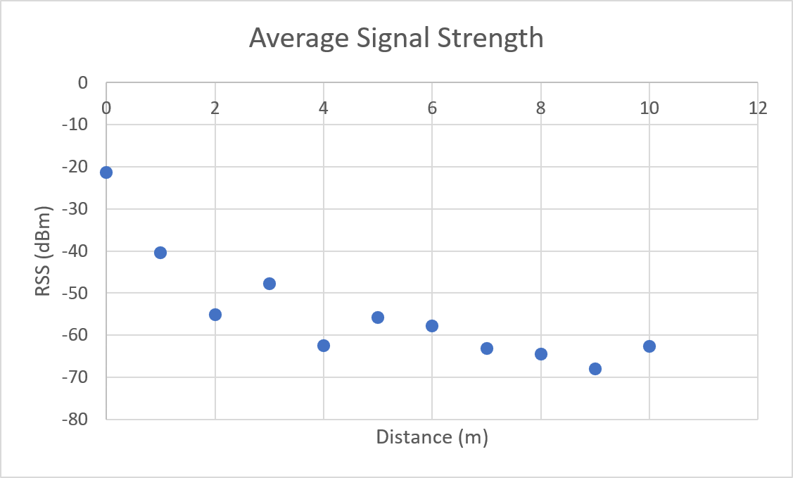 | |
Table 1
| Distance (m) | Average RSS (dBm) | Min RSS (dBm) | Max RSS (dBm) | RSS Range (dBm) | # Data Points |
|---|---|---|---|---|---|
| 0 | -21.32 | -30 | -16 | 14 | 584 |
| 1 | -40.47 | -48 | -40 | 8 | 631 |
| 2 | -55.18 | -68 | -44 | 24 | 670 |
| 3 | -49.71 | -56 | -48 | 8 | 711 |
| 4 | -62.47 | -68 | -50 | 18 | 692 |
| 5 | -55.78 | -64 | -50 | 14 | 678 |
| 6 | -57.84 | -68 | -52 | 16 | 668 |
| 7 | -63.09 | -74 | -50 | 24 | 691 |
| 8 | -64.46 | -74 | -52 | 22 | 655 |
| 9 | -67.92 | -78 | -56 | 22 | 662 |
| 10 | -62.67 | -74 | -56 | 18 | 540 |
Analysis
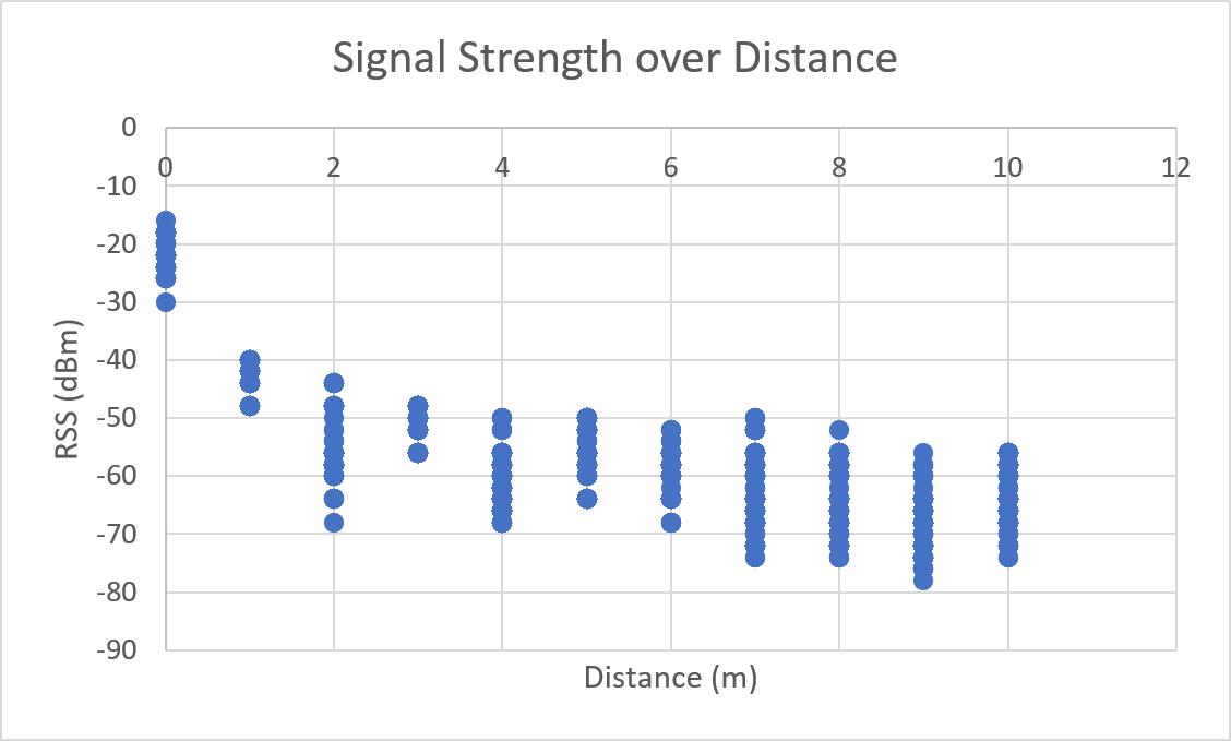
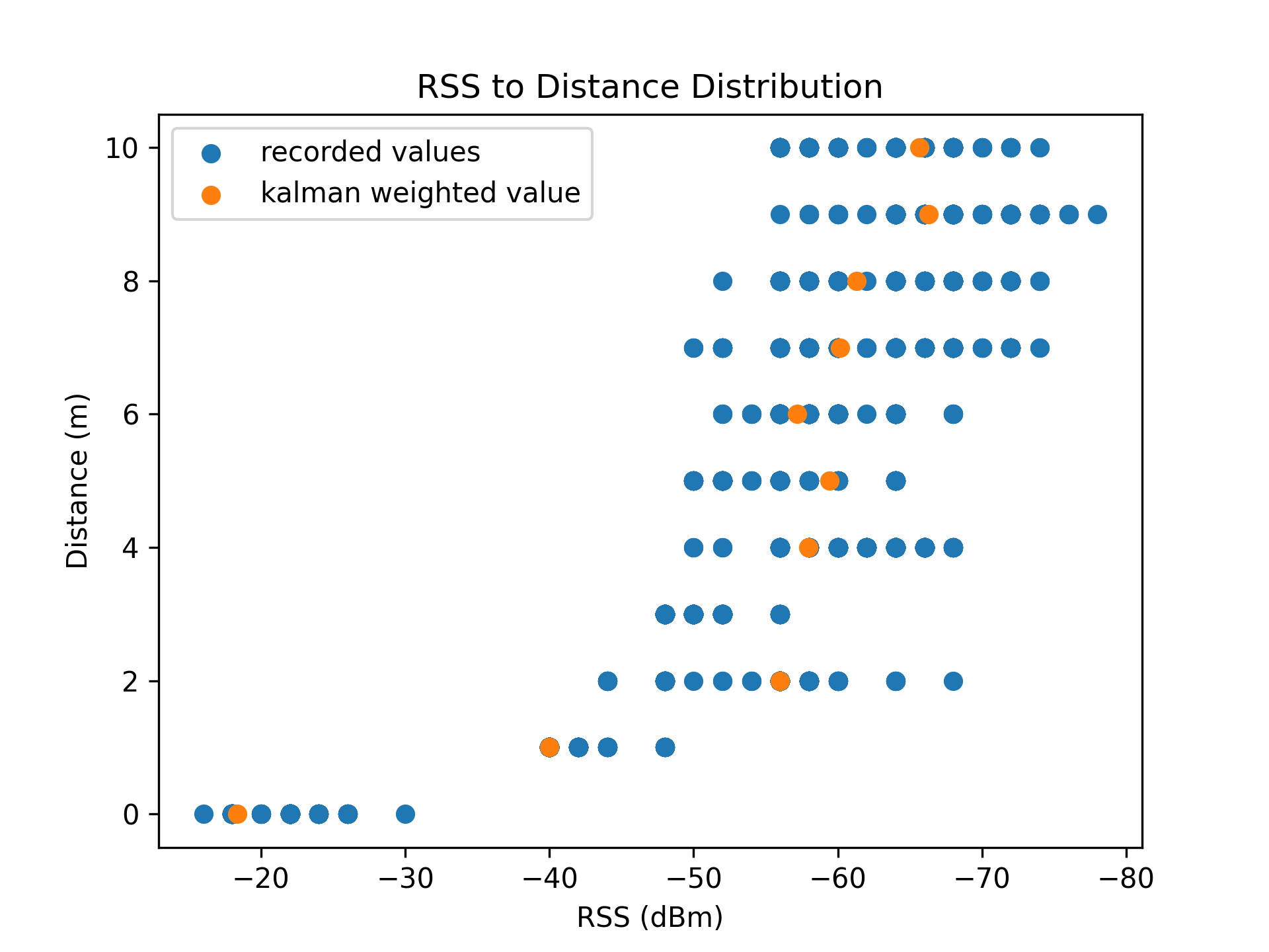
As a result of environmental factors, the recorded values have been affected by induced atmospheric noise, and interference from other electrical signals. These fluctuations are evident through the range of different RSS values in each distance class (See [Table 1]).
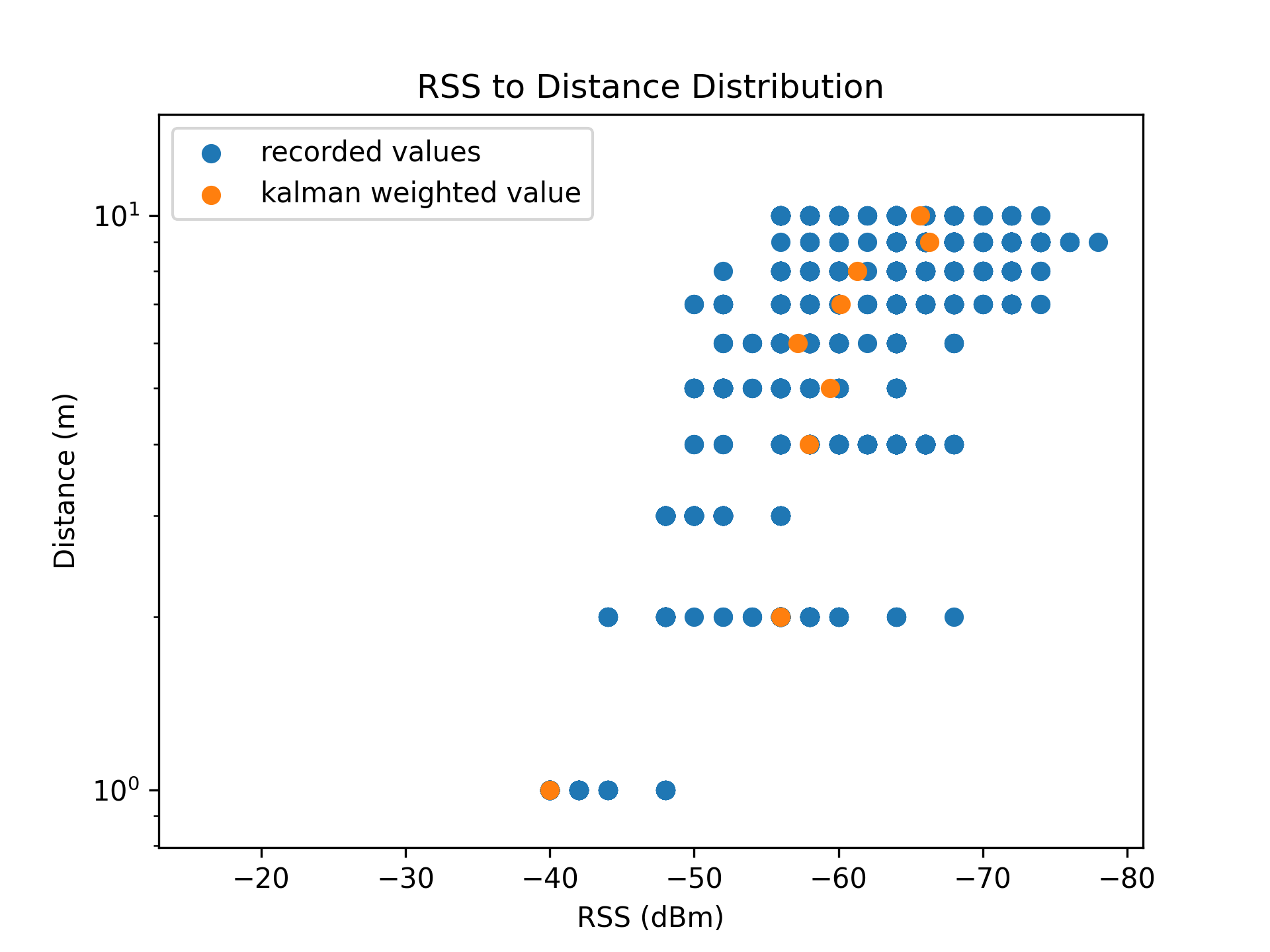
Kalman Filter
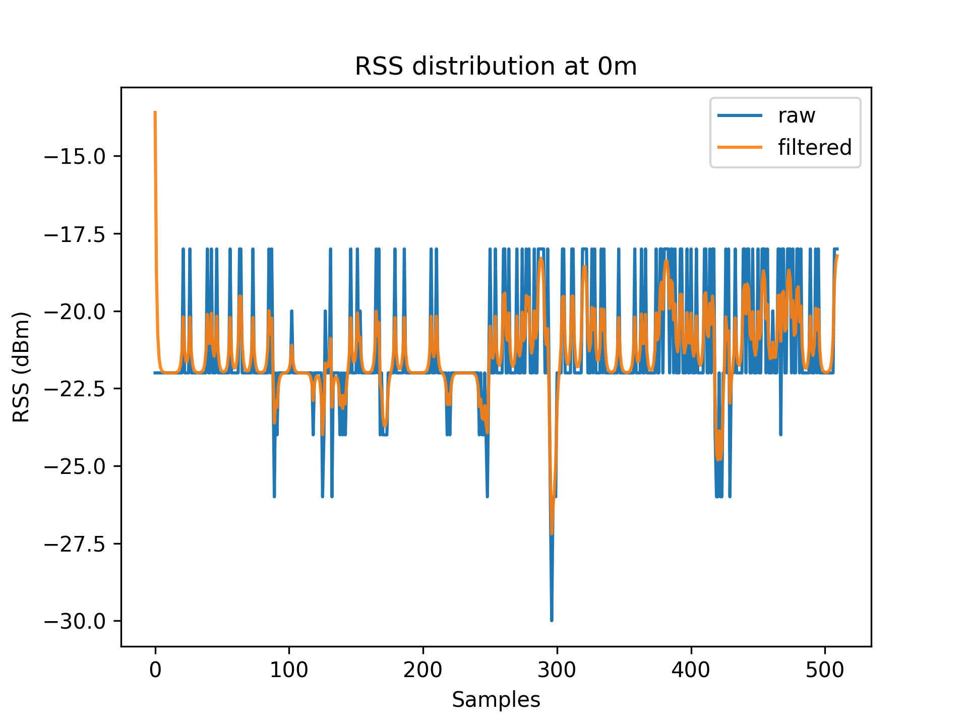
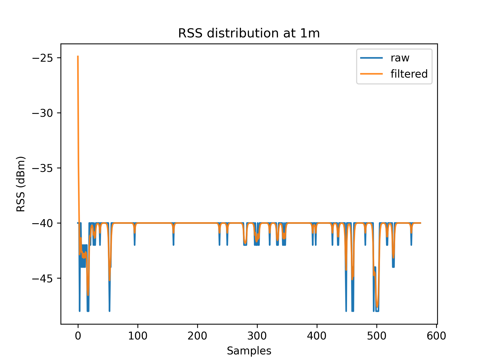
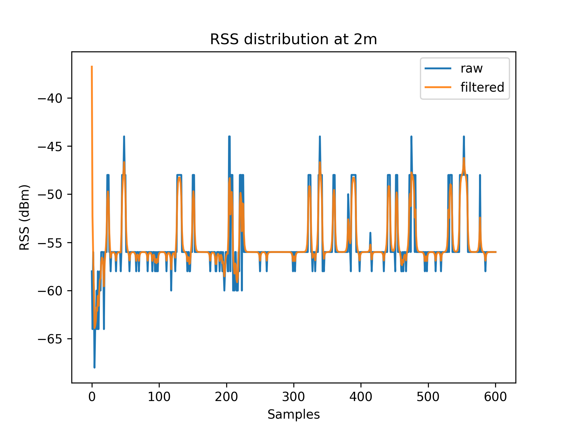
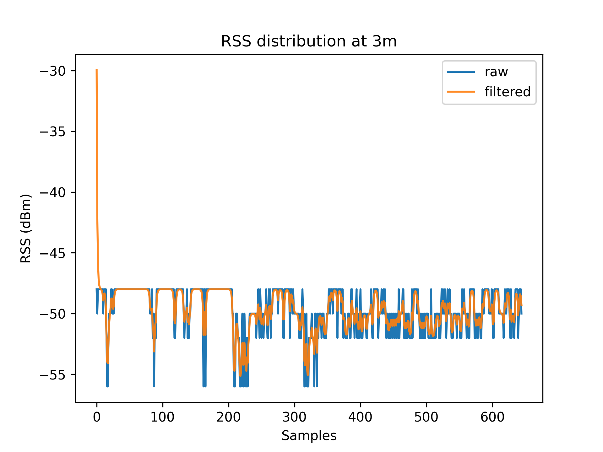
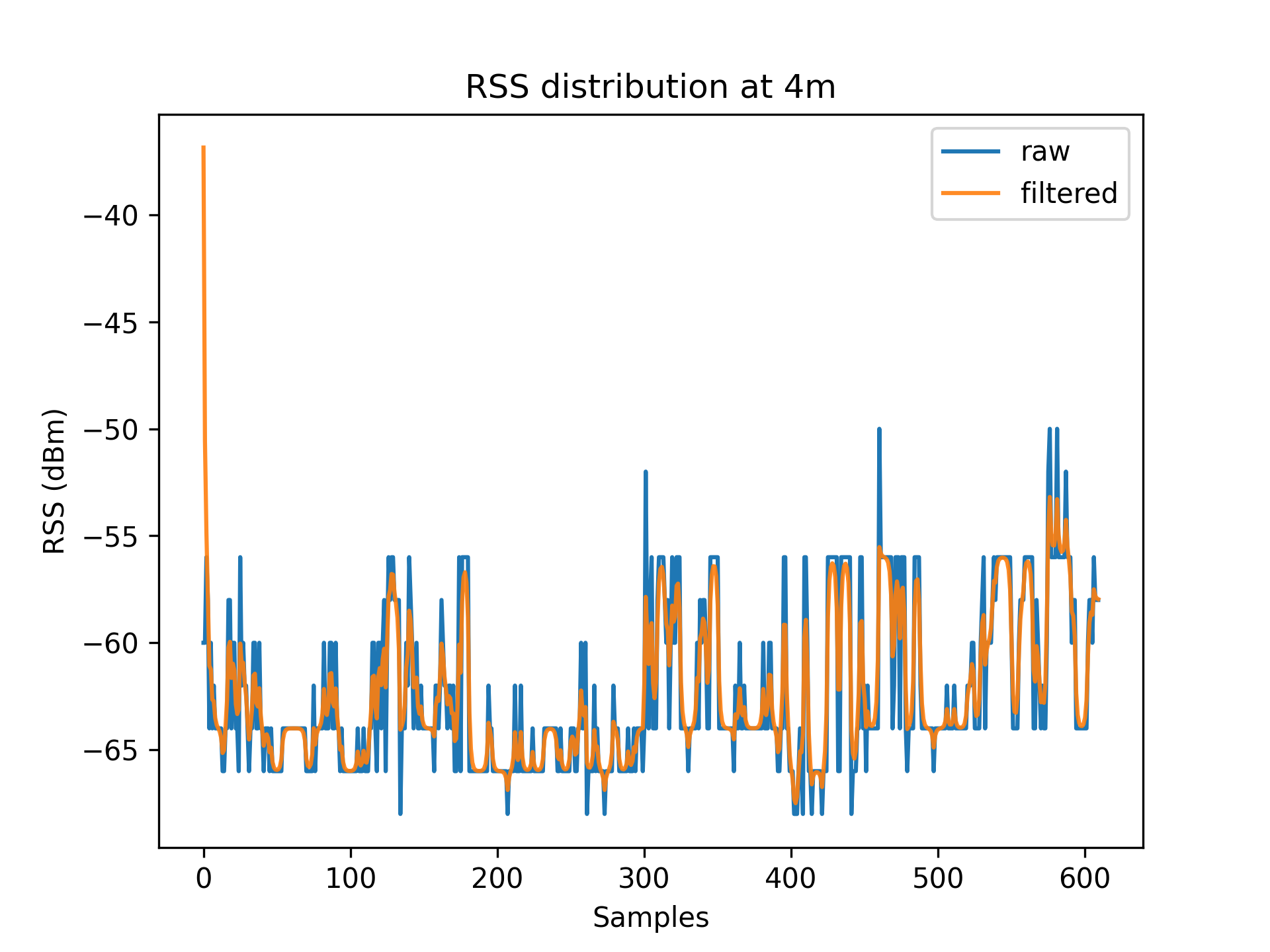
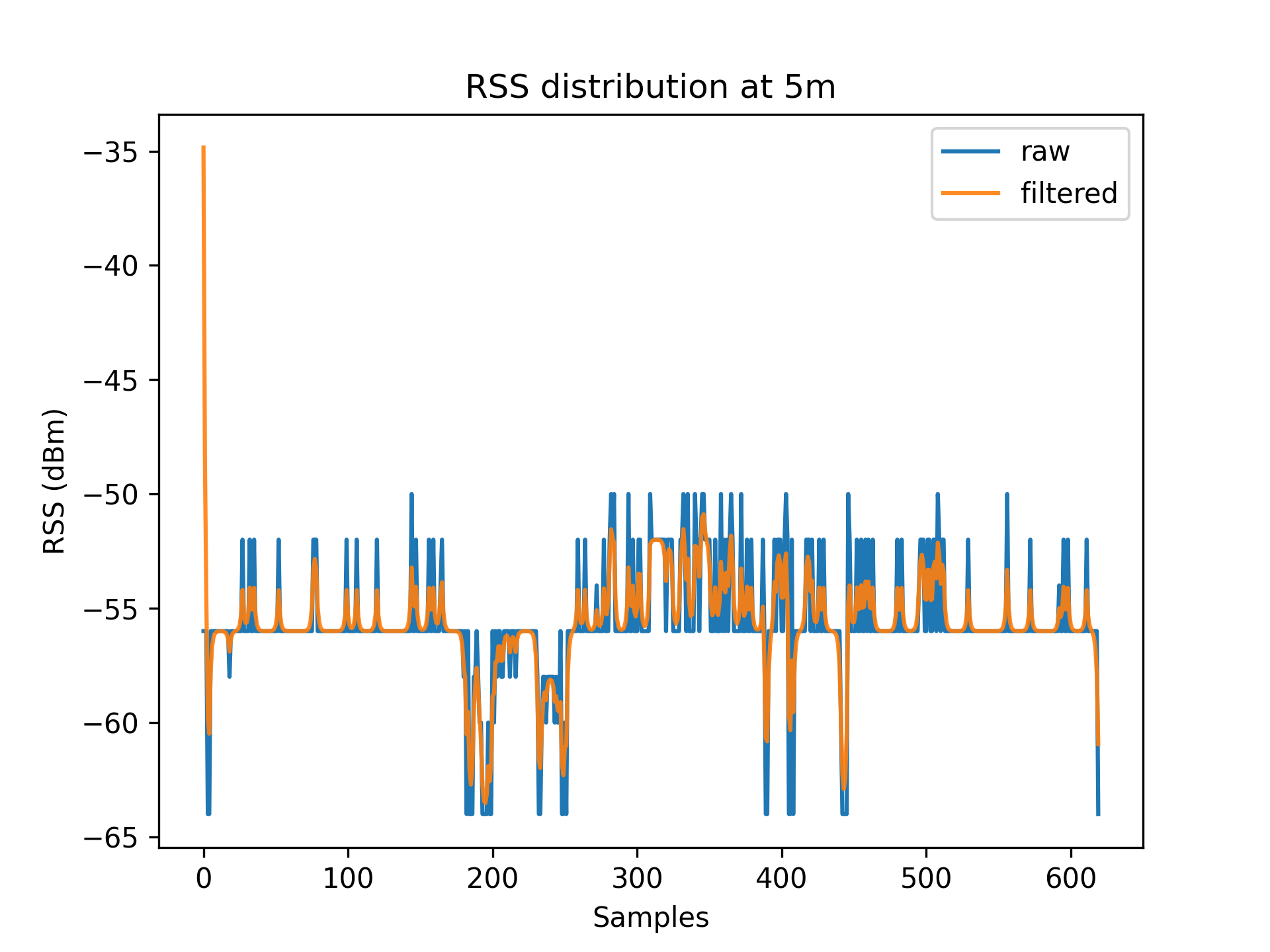
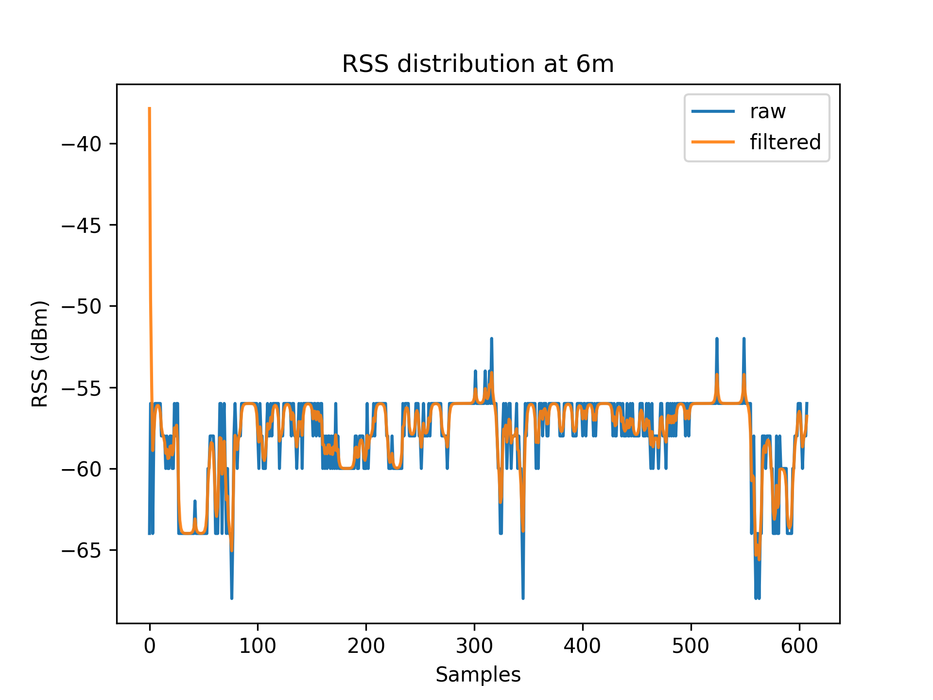
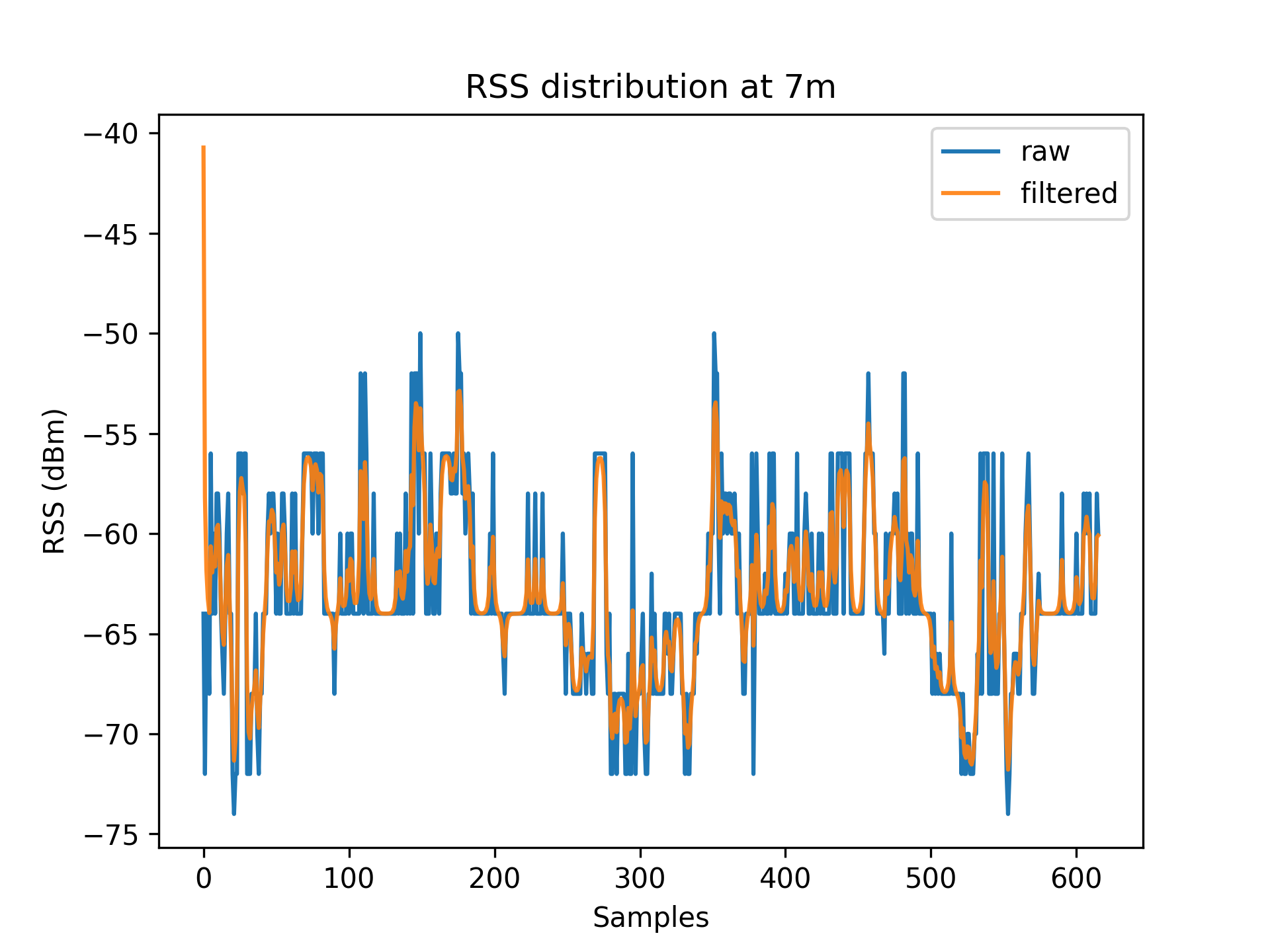
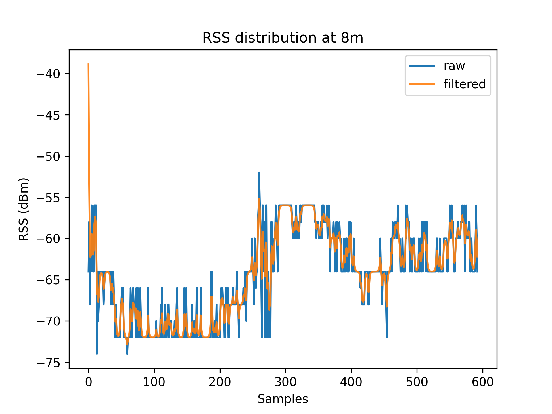
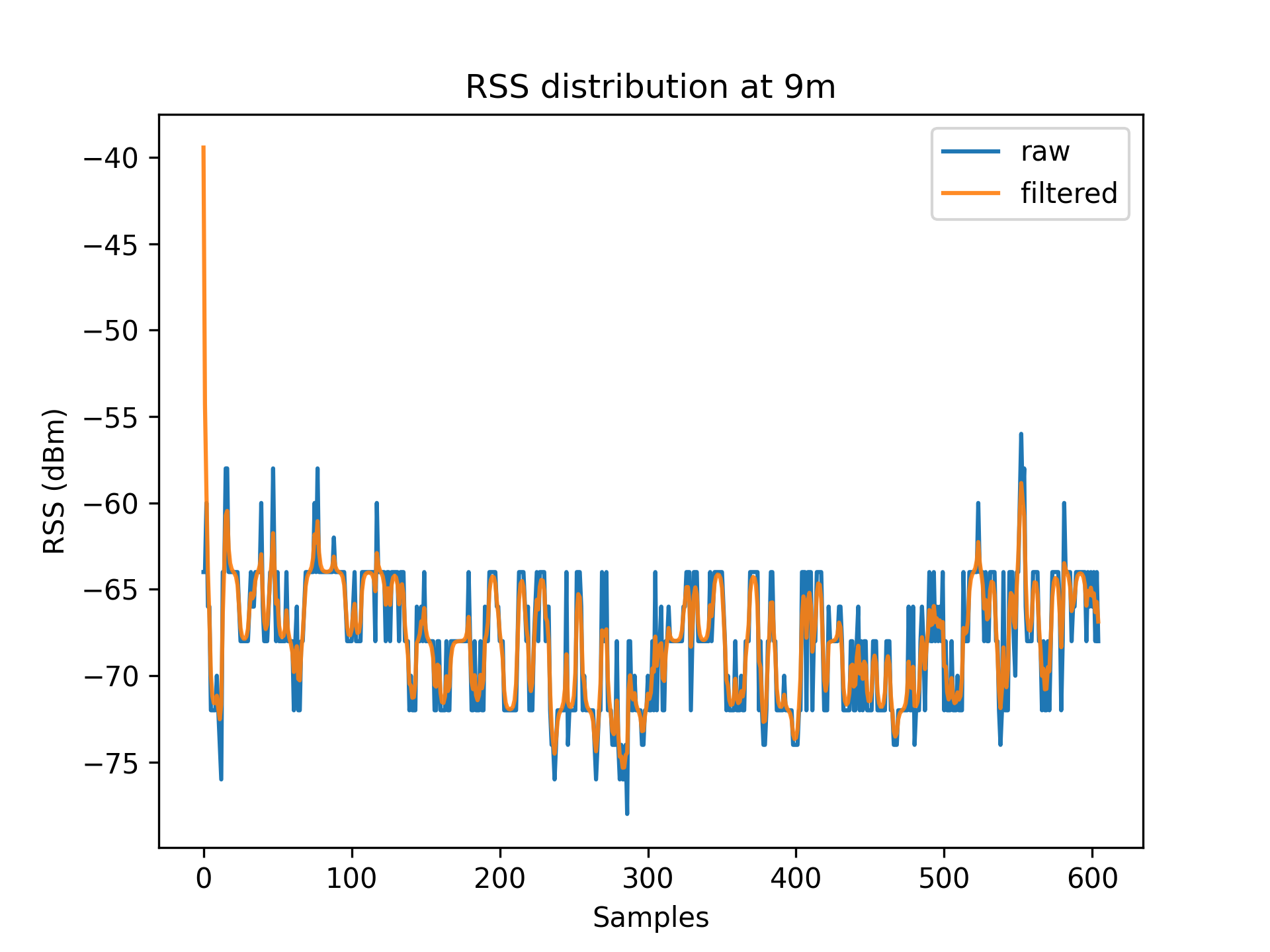
To account for RSS fluctuations, a $Kalman\ filter$ can be applied on each distance set.
The application of the Kalman filter produces a series of points which have a lower range and variance.
Figures 3.1 to 3.11 display the decreased RSS variance as a result of the Kalman filter process.
| Graph |
|---|
 |
 |
 |
 |
 |
 |
 |
 |
 |
 |
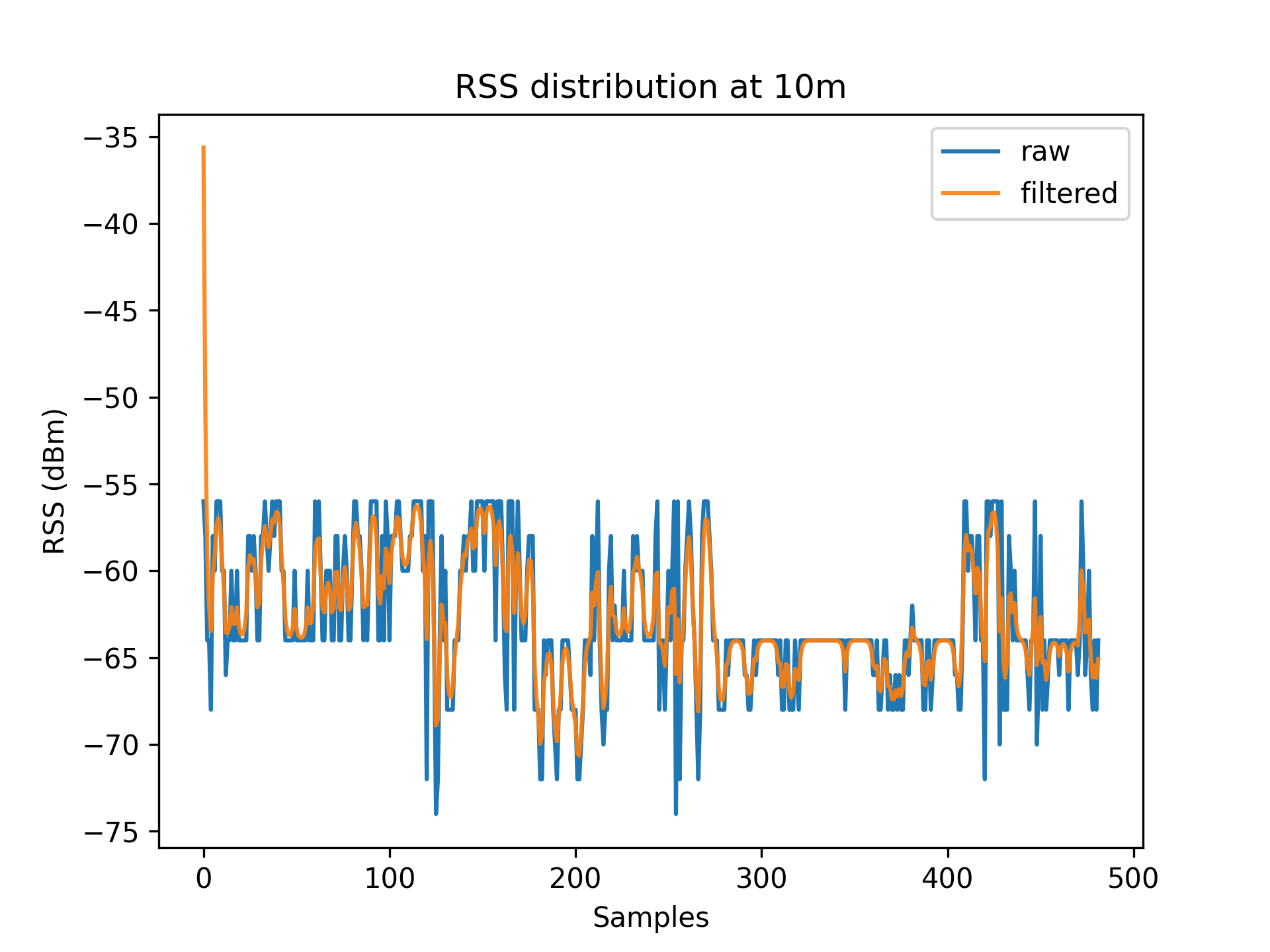 |
Table 2
| Distance (m) | RSS Range - no filter (dBm) | RSS Range - Kalman filter (dBm) |
|---|---|---|
| 0 | 14 | 8.87 |
| 1 | 8 | 7.13 |
| 2 | 24 | 18.18 |
| 3 | 8 | 7.47 |
| 4 | 18 | 14.98 |
| 5 | 14 | 12.83 |
| 6 | 16 | 11.53 |
| 7 | 24 | 18.66 |
| 8 | 22 | 17.69 |
| 9 | 22 | 16.98 |
| 10 | 18 | 14.51 |
Set Removal
| Linear Average | Logarithmic Average |
|---|---|
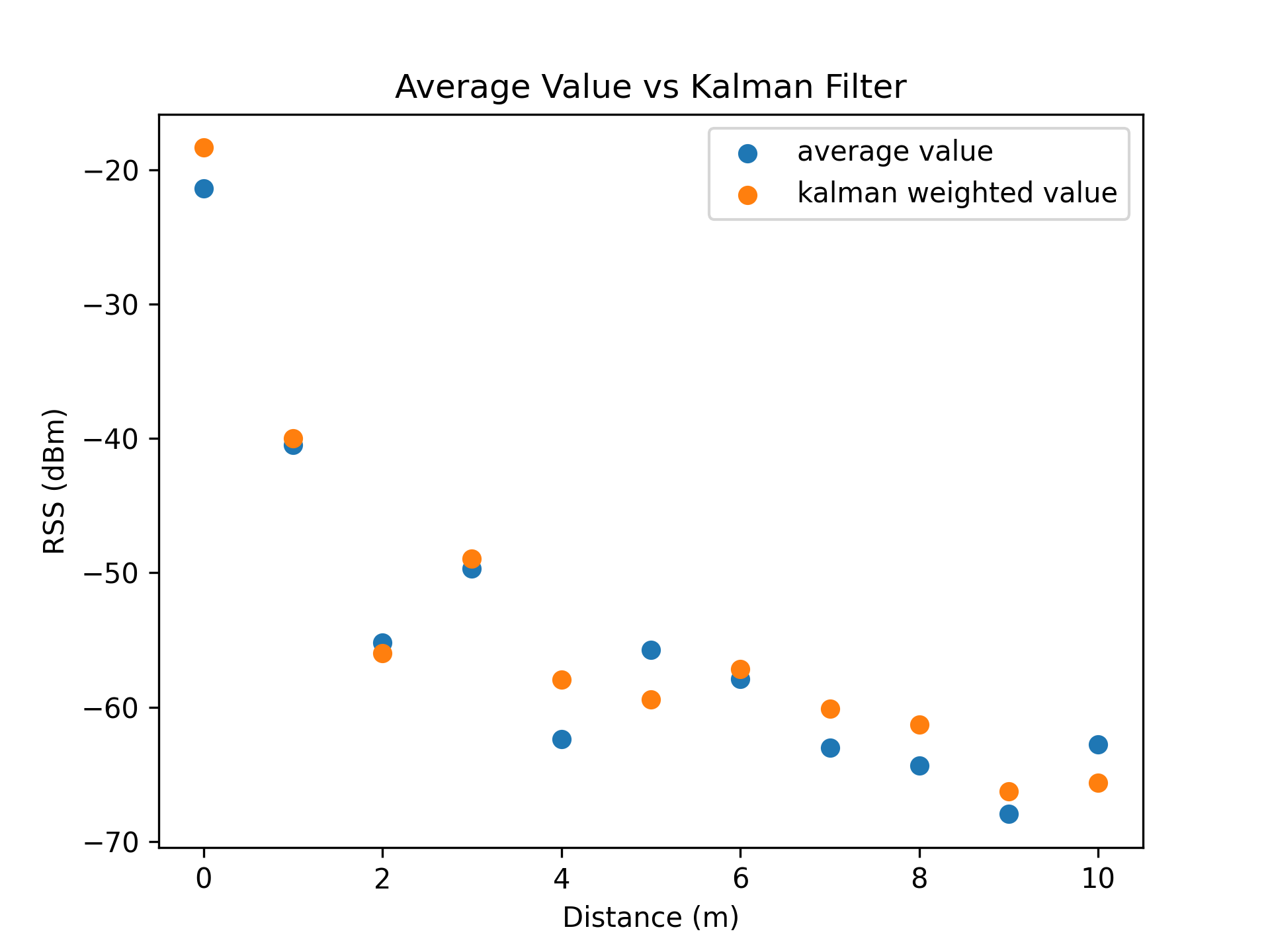 |  |
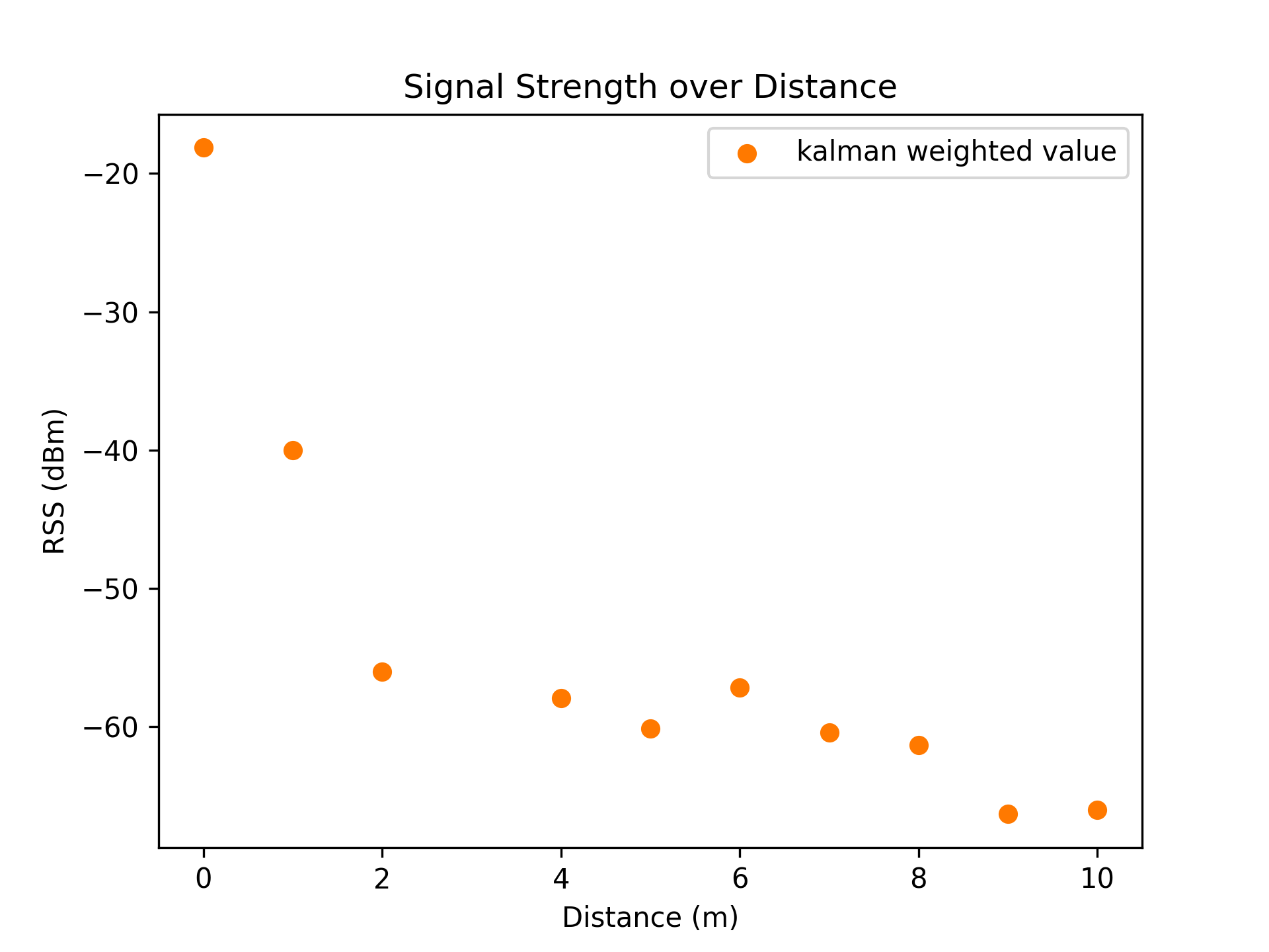
Considering a WiFi network broadcasted by a single access point, the series of recorded signal strengths and their averages should follow a strictly decreasing trend. This is due to the principle that electromagnetic waves experience exponential decay, proportional to the distance travelled.
However, as seen in [Figure 4.1] and [Figure 4.2] the set of recorded RSS values at distance 3 meters have an abnormally high average value, and should be removed as an outlier group.
Testament to the fact that the variation in RSS values is very low (The data set had an RSS range of 8 dBm), it is likely that this outcome had occurred due to spatial environmental factors. Upon examination of the testing location, the location marked three meters away from the access point was beside an open area of space. Consequently, the effects of multipath transmission would have been lowered, hence resulting in all recorded values (of that distance group) having a significantly higher signal strength.
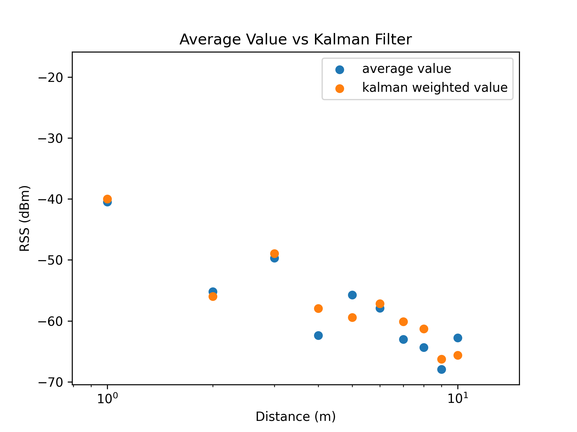
This observation may also be loosely applied to the set of RSS values recorded at distances of 6 and 10 meters, which share similar spatial properties.
| Linear Average | Logarithmic Average |
|---|---|
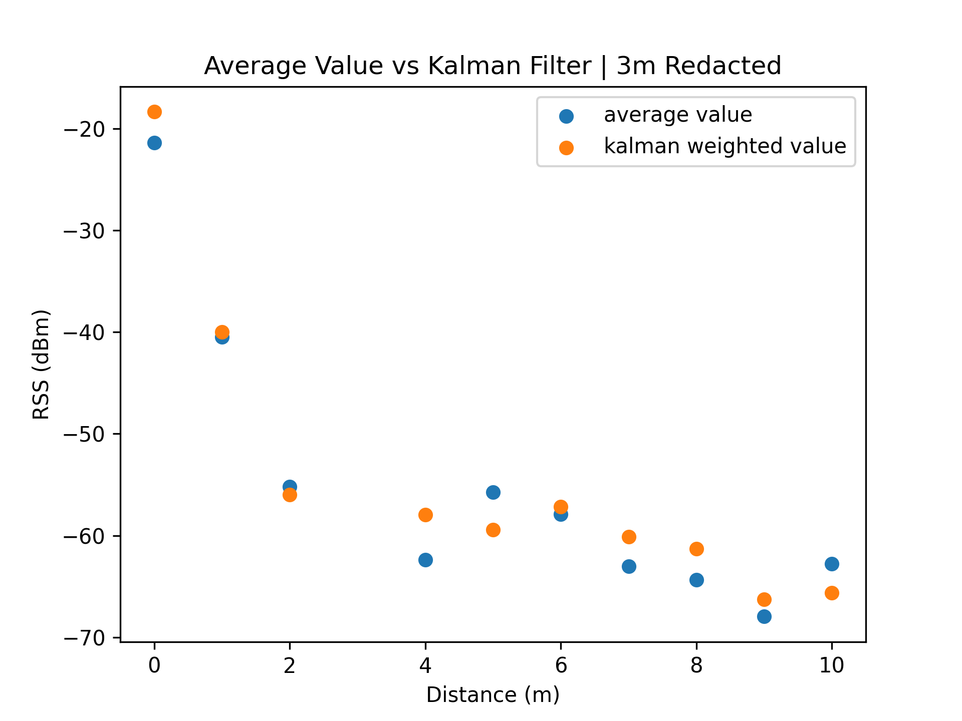 | 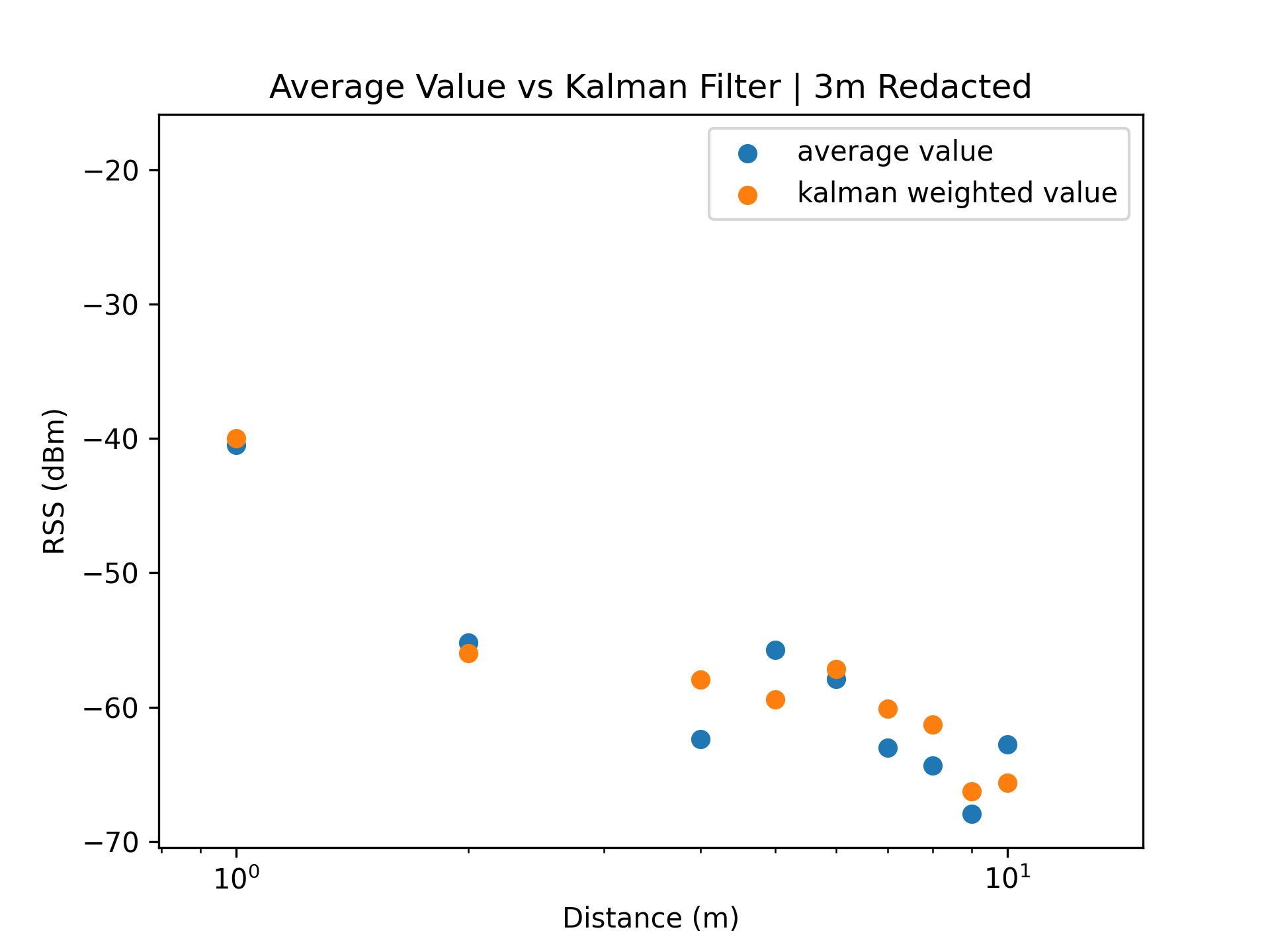 |
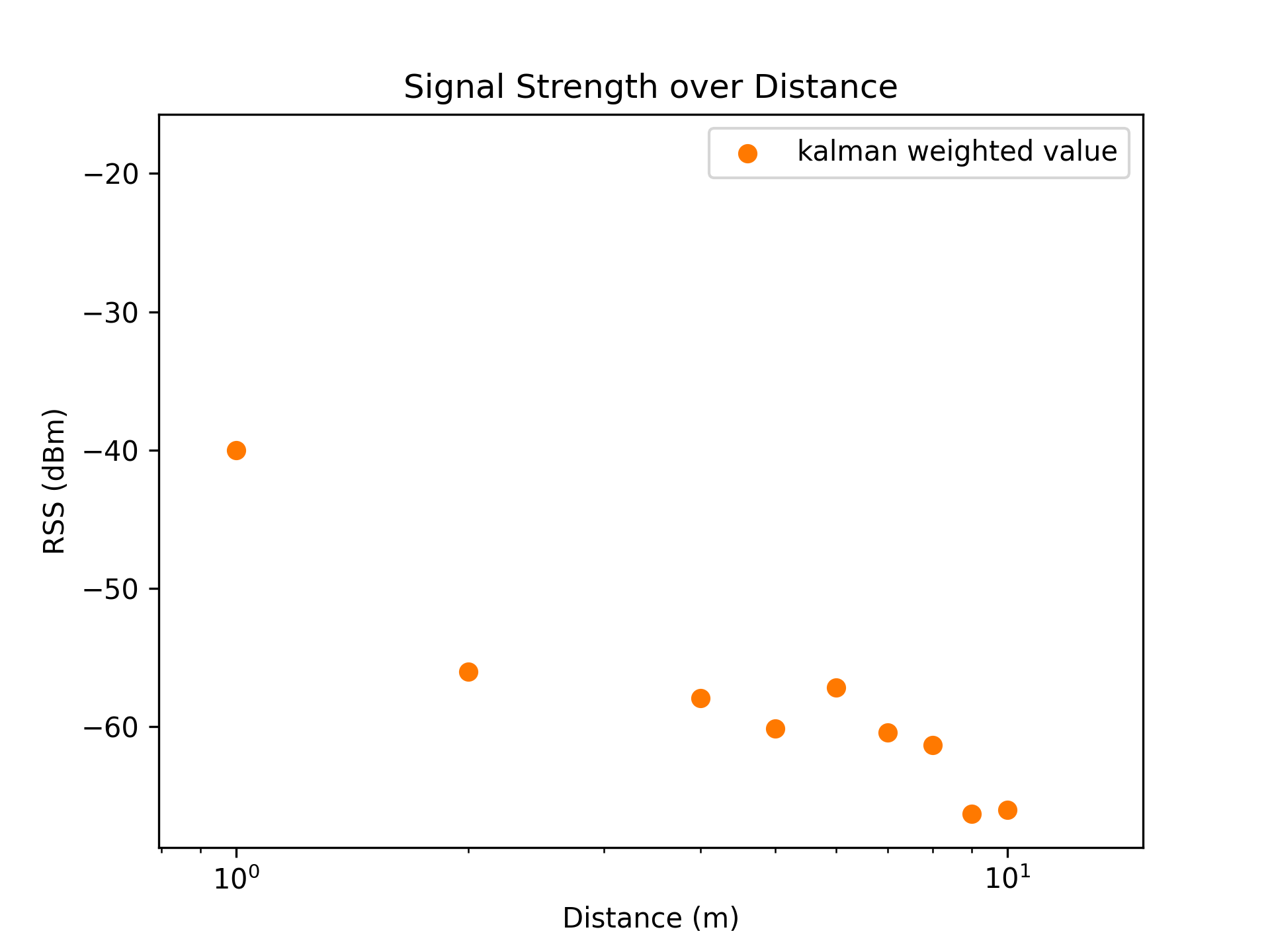
Removing the outlier group at distance 3m, the series of RSS values better follow a logarithmic decline.
The Kalman filter result set now has a cleaner series of data which we can perform analysis on.
| Linear Average | Logarithmic Average |
|---|---|
 |  |
Data Fitting
The log distance path loss model describes the power loss (in decibels) of a signal as a result of distance separation. It is defined as the following
$$ PL(d) = PL({d_0}) + 10 \times n \times log_{10}(\frac{d}{d_0}) + \chi $$ $$ for\ d_0 \le d $$
- $PL(...)$ is the path loss at a given distance
- $d$ is the distance between the antenna and receiver
- $d_0$ is a reference distance
- $n$ is the path loss exponent
- $\chi$ is a zero mean Gaussian random variable (For consideration of signal shadowing)
This model can be rewritten to produce an expression describing the distance required to achieve a given power loss.
$$d(PL) = \Large e^{\frac{PL_{d_0} + PL + \chi}{10 \times n}}$$
- $PL$ is the path loss
- $PL_{d_0}$ is the path loss at distance $d_0$
- $d_0$ is a reference distance
- $n$ is the path loss exponent
- $\chi$ is a zero mean Gaussian random variable (For consideration of signal shadowing)
This expression ( $y(x) = e^x$ ) suits the trend of the data, when the axes are flipped.
| Linear Scale | Logarithmic Scale |
|---|---|
 |  |
To determine $\chi$ and $n$, the curve_fit function of the scipy library was used on the sample data.
The reference distance $d_0$ was set to $1\ m$, resulting in $PL_{d_0} = -40\ dB$.
The curve fitting function produced the values $\chi = 0.37$ and $n = 1.15$.
$$\Large distance = e^{\frac{-40.0 + RSS + 0.37}{10 \times 1.15}}$$
| Linear Scale | Logarithmic Scale |
|---|---|
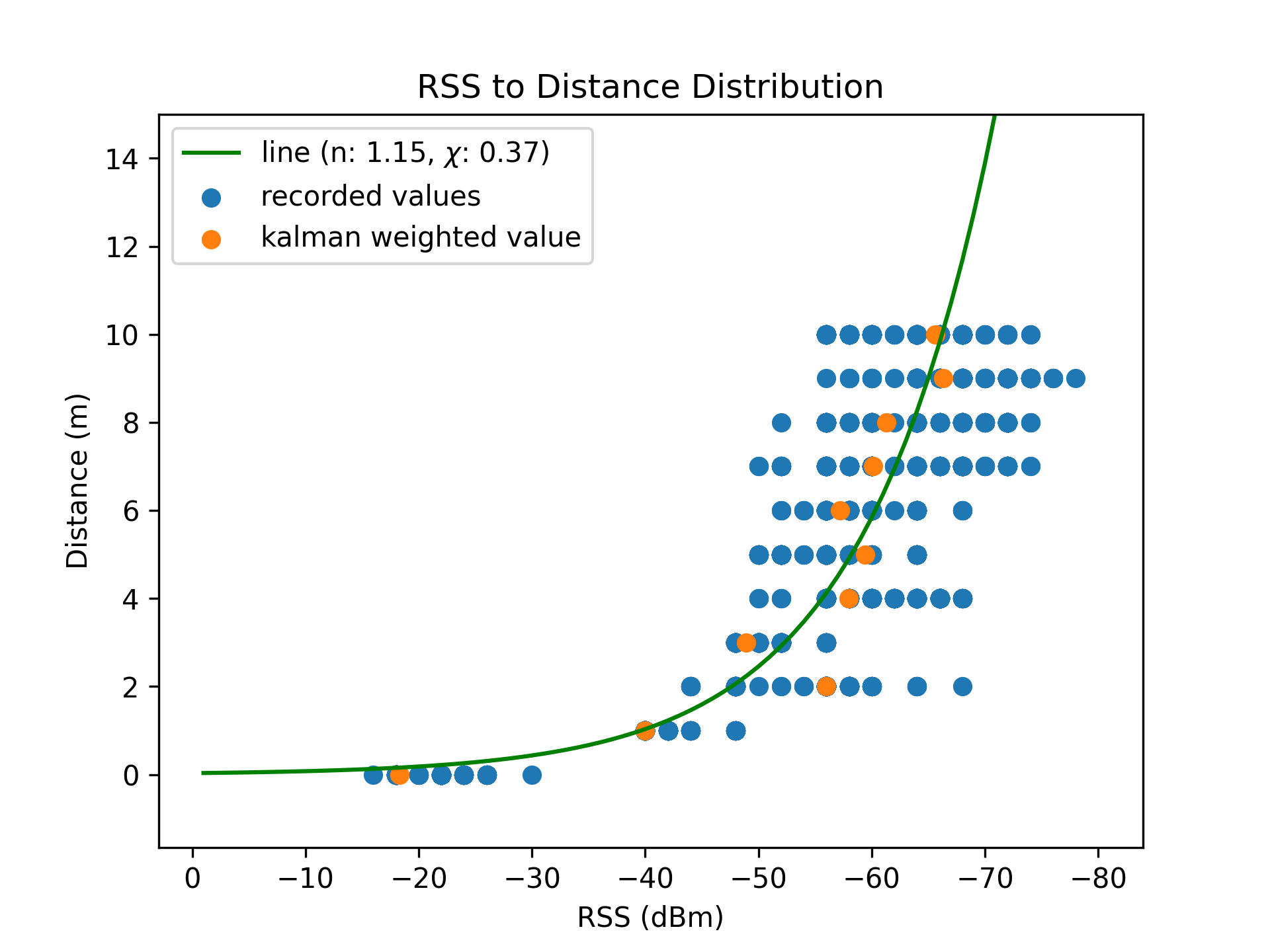 | 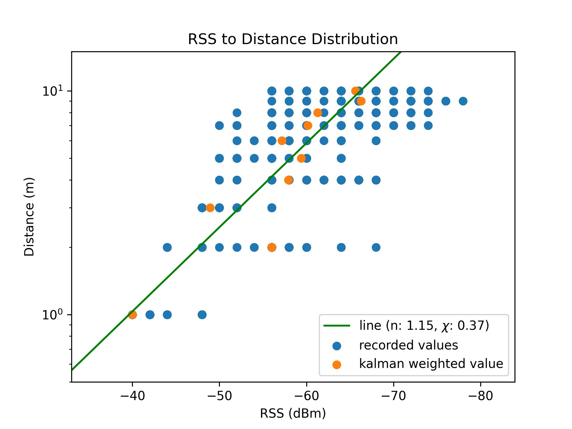 |
[Figure 8.1] and [Figure 8.2] superimpose the derived distance approximation model on the training sample set, revealing a strong coefficient of determination $R^2 = 0.88$. This is an improvement over the score of $R^2 = 0.62$ for the naive preliminary algorithm.
Testing
Distance approximation formula: $\large d = e^{\frac{-40.0 + RSS + 0.37}{10 \times 1.15}}$
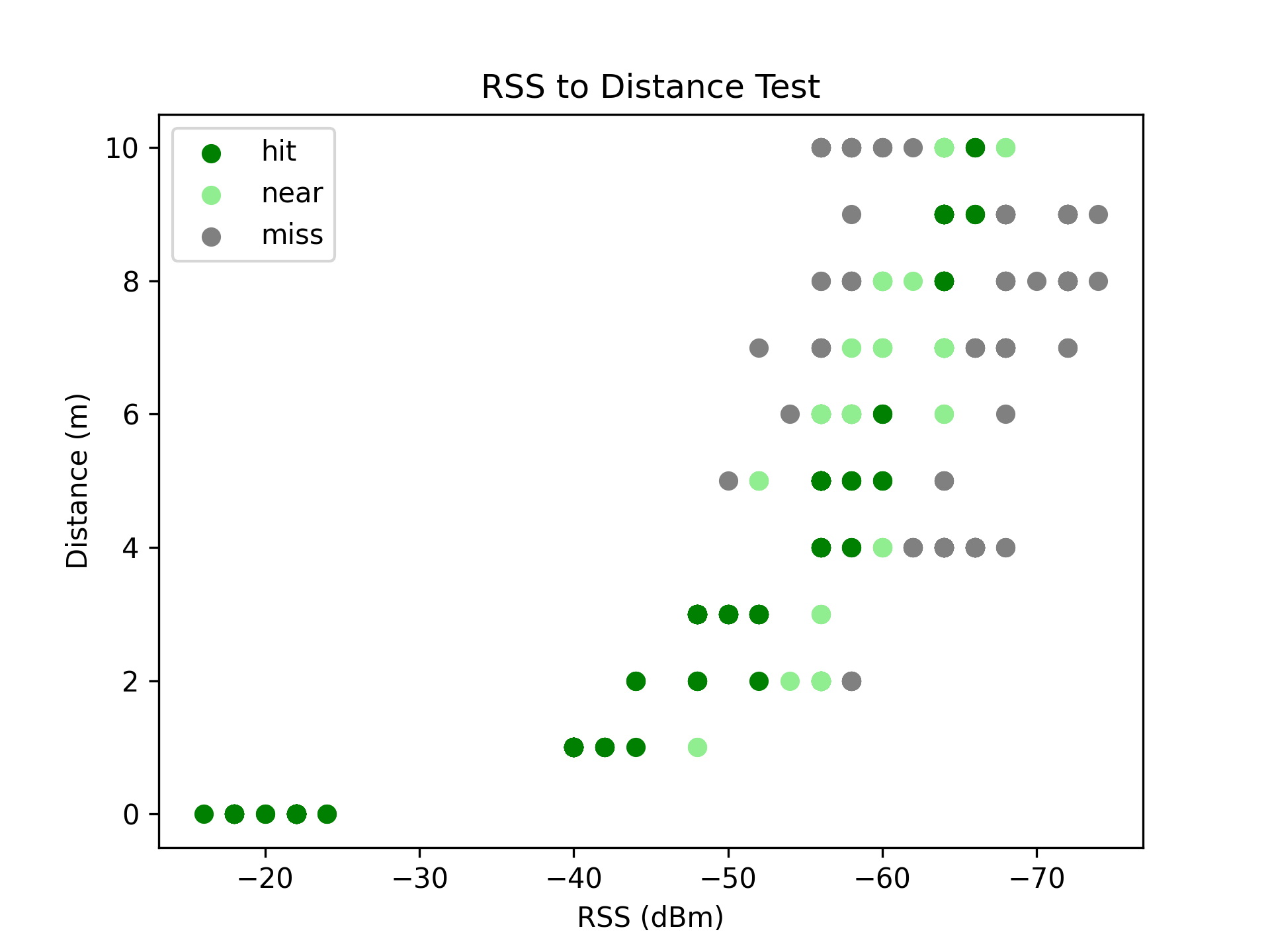
When applying the distance approximation on the test samples, an overall hit-rate of 72.28% was obtained.
519 of the 718 samples approximated the correct distance within a 1 meter tolerance.
This algorithm has a noticeably higher performance compared to the naive algorithm, as all test sample classes had at least one distance match.
Table 3
| Naive Method | Log Distance Method | |
|---|---|---|
| Formula | $d = -\frac{RSS+38.521}{3.303}$ | $d = e^{\frac{-40.0 + RSS + 0.37}{10 \times 1.15}}$ |
| $R^2$ Score | 0.62 | 0.88 |
| Hit-rate at 0m | 0% | 100.0% |
| Hit-rate at 1m | 35.85% | 100.0% |
| Hit-rate at 2m | 0% | 89.86% |
| Hit-rate at 3m | 0% | 100.0% |
| Hit-rate at 4m | 15.09% | 25.61% |
| Hit-rate at 5m | 59.09% | 91.38% |
| Hit-rate at 6m | 2.94% | 96.67% |
| Hit-rate at 7m | 86.57% | 58.67% |
| Hit-rate at 8m | 1.75% | 40.32% |
| Hit-rate at 9m | 2.33% | 42.11% |
| Hit-rate at 10m | 10.42% | 60.34% |
Conclusion
This experiment aimed to find a universal and portable method of determining distances between two devices.
The extrapolated model follows the algorithm: $\large d = e^{\frac{-40.0 + RSS + 0.37}{10 \times 1.15}}$
Whilst not a universal solution to all wireless environments, it is portable and easily recalculable.
RSSI values are not the most optimal measurement of distance, due to their influence from many environment factors.
However, results drawn from this experiment conclude that it is definitely possible to use RSSI values to produce an estimated distance - within reasonable accuracy.
As wireless devices do not receive just one, but hundreds and thousands of packets, further distance accuracy can be gained by continually applying a Kalman filter on all of the incoming RSS values.
As seen from analysis, the Log-Distance Path Model better represents the signal strength response to distance separation when compared to the naive distance estimation approach - which modelled a linear equation. The incorporation of a Kalman filter reduced the variance of recorded RSS values in each distance class, which further improved the performance and accuracy of the model.
References
- A Mobile App for Real-Time Testing of Path-Loss Models and Optimization of Network Planning
- Determining the relative position of a device in a wireless network with minimal effort, 2016
- Enhancements to rss based indoor tracking systems using kalman filters, 2003
- GaussianWaves. 2020. Log Distance Path Loss Or Log Normal Shadowing Model
- Kalman filters explained: Removing noise from RSSI signals
- KNN Classification
- Li G, Geng E, Ye Z, et al. Indoor Positioning Algorithm Based on the Improved RSSI Distance Model. Sensors (Basel, Switzerland). 2018 Aug;18(9). DOI: 10.3390/s18092820.
- Open Journal of Internet Of Things, 2015. Accurate Distance Estimation Between Things: A Self-correcting Approach. 1(2)
- PyKalman
- Using RSSI value for distance estimation in Wireless sensor networks based on ZigBee, 2000
Apendices
Program Trace
$> python3 grab.py

Averages: -21.37 -40.46 -55.2 -49.7 -62.41 -55.72 -57.89 -63.0 -64.35 -67.96 -62.76
Kalman Averages: -18.33 -40.0 -56.0 -48.92 -57.94 -59.41 -57.18 -60.14 -61.29 -66.3 -65.63
RSS Range: 12 8 24 8 18 14 16 24 22 22 18
RSS Range (Kalman): 13.6 22.72 27.13 25.19 30.64 28.68 27.77 31.06 33.98 35.89 35.01
distance = exp( (-40.0 + RSS + 0.37) / (10*1.15) )
R^2 = 0.88

Hit-rate for 0m :: 74/74 :: 100.0%
Hit-rate for 1m :: 57/57 :: 100.0%
Hit-rate for 2m :: 62/69 :: 89.86%
Hit-rate for 3m :: 66/66 :: 100.0%
Hit-rate for 4m :: 21/82 :: 25.61%
Hit-rate for 5m :: 53/58 :: 91.38%
Hit-rate for 6m :: 58/60 :: 96.67%
Hit-rate for 7m :: 44/75 :: 58.67%
Hit-rate for 8m :: 25/62 :: 40.32%
Hit-rate for 9m :: 24/57 :: 42.11%
Hit-rate for 10m :: 35/58 :: 60.34%

Total hit-rate :: 519/718 :: 72.28%
Analysis Script
Data Sets
- Indoor measurements - [indoor.zip]
- Outdoor measurements - [outdoor.zip]